3. THE DATUM AND THE EARTH AS AN ELLIPSOID #
For many maps, including nearly all maps in commercial atlases, it may be assumed that the Earth is a sphere. Actually, it is more nearly an oblate ellipsoid of revolution, also called an oblate spheroid. This is an ellipse rotated about its shorter axis. The flattening of the ellipse for the Earth is only about one part in three hundred; but it is sufficient to become a necessary part of calculations in plotting accurate maps at a scale of 1:100,000 or larger, and is significant even for 1:5,000,000-scale maps of the United States, affecting plotted shapes by up to 213 percent (see p. 27). On small-scale maps, including single-sheet world maps, the oblateness is negligible. Formulas for both the sphere and ellipsoid will be discussed in this book wherever the projection is used or is suitable in both forms. The Earth is not an exact ellipsoid, and deviations from this shape are continually evaluated. The geoid is the name given to the shape that the Earth would assume if it were all measured at mean sea level. This is an undulating surface that varies not more than about a hundred meters above or below a well-fitting ellipsoid, a variation far less than the ellipsoid varies from the sphere. It is important to remember that elevations and contour lines on the Earth are reported relative to the geoid, not the ellipsoid. Latitude, longitude, and all plane coordinate systems, on the other hand, are determined with respect to the ellipsoid.
The choice of the reference ellipsoid used for various regions of the Earth has been influenced by the local geoid, but large-scale map projections are designed to fit the reference ellipsoid, not the geoid. The selection of constants defining the shape of the reference ellipsoid has been a major concern of geodesists since the early 18th century. Two geometric constants are sufficient to define the ellipsoid itself. They are normally expressed either as (1) the semimajor and semiminor axes (or equatorial and polar radii, respectively), (2) the semimajor axis and the flattening, or (3) the semimajor axis and the eccentricity. These pairs are directly interchangeable. In addition, recent satellite-measured reference ellipsoids are defined by the semimajor axis, geocentric gravitational constant, and dynamical form factor, which may be converted to flattening with formulas from physics (Lauf, 1983, p. 6).
In the early 18th century, Isaac Newton and others concluded that the Earth should be slightly flattened at the poles, but the French believed the Earth to be egg-shaped as the result of meridian measurements within France. To settle the matter, the French Academy of Sciences, beginning in 1735, sent expeditions to Peru and Lapland to measure meridians at widely separated latitudes. This established the validity of Newton’s conclusions and led to numerous meridian measurements in various locations, especially during the 19th and 20th centuries; between 1799 and 1951 there were 26 determinations of dimensions of the Earth.
The identity of the ellipsoid used by the United States before 1844 is uncertain, although there is reference to a flattening of 1/302. The Bessel ellipsoid of 1841 (see table 1) was used by the Coast Survey from 1844 until 1880, when the bureau adopted the 1866 evaluation by the British geodesist Alexander Ross Clarke using measurements of meridian arcs in western Europe, Russia, India, South Africa, and Peru (Shalowitz, 1964, p. 117-118; Clarke and Helmert, 1911, p. 807-808). This resulted in an adopted equatorial radius of 6,378,206.4 m and a polar radius of 6,356,583.8 m, or an approximate flattening of 1/294.9787.
The Clarke 1866 ellipsoid (the year should be included since Clarke is also known for ellipsoids of 1858 and 1880) has been used for all of North America until a change which is currently underway, as described below.
In 1909 John Fillmore Hayford reported calculations for a reference ellipsoid from U.S. Coast and Geodetic Survey measurements made entirely within the United States. This was adopted by the International Union of Geodesy and Geophysics (IUGG) in 1924, with a flattening of exactly 1/297 and a semimajor axis of exactly 6,378,388 m. This is therefore called the International or the Hayford ellipsoid, and is used in many parts of the world, but it was not adopted for use in North America, in part because of all the work already accomplished using the older datum and ellipsoid (Brown, 1949, p. 293; Hayford, 1909).
| Name | Date | Equatorial Radius, a (meters) | Polar Radius, b (meters) | Flattening | Use |
|---|---|---|---|---|---|
| GRS 802 | 1980 | 6378137 | 6356752.3 | 1/298.257 | Newly adopted |
| WGS 723 | 1972 | 6378135 | 6356750.5 | 1/298.26 | NASA; Dept. of Defense;oil companies |
| Australian | 1965 | 6378160 | 6356774.7 | 1/298.25 | Australia |
| Krassovsky | 1940 | 6378245 | 6356863.0 | 1/298.3 | Soviet Union |
| International | 1924 | 6378388 | 6356911.0 | 1/297 | Reminder of the world† |
| Hayford | 1909 | ||||
| Clarke4 | 1880 | 6378249.1 | 6356514.9 | 1/293.32 | Most of Africa; France |
| Clarke | 1866 | 6378206.4 | 6356583.8 | 1/294.98 | North America; Philippines |
| Airy | 1830 | 6377563.4 | 6356256.9 | 1/299.32 | Great Britain |
| Bessel | 1841 | 6377397.2 | 6356079.0 | 1/299.15 | Central Europe; Chile; Indonesia |
| Everest | 1830 | 6377276.3 | 6356075.4 | 1/300.80 | India; Burma; Pakistan; Afghanistan; Thailand; etc. |
| Values are shown to accuracy in excess
significant figures, to reduce computational confusion. 1 Mahng, 1973, p. 7; Thomas, 1970, p. 84; Army, 1973, p. 4, endmap; Colvocoresses, 1969, p. 33; World Geodetic, 1974. 2 Geodetic Reference System. Ellipsoid derived from adopted model of Earth. WGS 84 has same dimensions within accuracy shown. 3World Geodetic System. Ellipsoid derived from adopted model of Earth. 4Also used in some regions with various modified constants. Taken as exact values. The third number (where two are asterisked) is derived using the following relationships: b = a (1-f); f = 1-(b/a). Where only one is asterisked (for 1972 and 1980), certain physical constants not shown are taken as exact, but f as shown is the adopted value. **Derived from a and b, which are rounded off as shown after conversions from lengths in feet. †Other than regions listed elsewhere in column, or some smaller areas. | |||||
There are over a dozen other principal ellipsoids, however, which are still used by one or more countries (table 1). The different dimensions do not only result from varying accuracy in the geodetic measurements (the measurements of locations on the Earth), but the curvature of the Earth’s surface (geoid) is not uniform due to irregularities in the gravity field.
Until recently, ellipsoids were only fitted to the Earth’s shape over a particular country or continent. The polar axis of the reference ellipsoid for such a region, therefore, normally does not coincide with the axis of the actual Earth, although it is assumed to be parallel. The same applies to the two equatorial planes. The discrepancy between centers is usually a few hundred meters at most. Only satellite-determined coordinate systems, such as the WGS 72 and GRS 80 mentioned below, are considered geocentric. Ellipsoids for the latter systems represent the entire Earth more accurately than ellipsoids determined from ground measurements, but they do not generally give the “best fit” for a particular region.
The reference ellipsoids used prior to those determined by satellite are related to an “initial point” of reference on the surface to produce a datum, the name given to a smooth mathematical surface that closely fits the mean sea-level surface throughout the area of interest. The “initial point” is assigned a latitude, longitude, elevation above the ellipsoid, and azimuth to some point. Once a datum is adopted, it provides the surface to which ground control measurements are referred. The latitude and longitude of all the control points in a given area are then computed relative to the adopted ellipsoid and the adopted “initial point.” The projection equations of large-scale maps must use the same ellipsoid parameters as those used to define the local datum; otherwise, the projections will be inconsistent with the ground control.
The first official geodetic datum in the United States was the New England Datum, adopted in 1879. It was based on surveys in the eastern and northeastern states and referenced to the Clarke Spheroid of 1866, with triangulation station Principio, in Maryland, as the origin. The first transcontinental arc of triangulation was completed in 1899, connecting independent surveys along the Pacific Coast. In the intervening years, other surveys were extended to the Gulf of Mexico. The New England Datum was thus extended to the south and west without major readjustment of the surveys in the east. In 1901, this expanded network was officially designated the United States Standard Datum, and triangulation station Meades Ranch, in Kansas, was the origin. In 1913, after the geodetic organizations of Canada and Mexico formally agreed to base their triangulation networks on the United States network, the datum was renamed the North American Datum.
By the mid-1920’s, the problems of adjusting new surveys to fit into the existing network were acute. Therefore, during the 5-year period 1927-1932 all available primary data were adjusted into a system now known as the North American 1927 Datum*** The coordinates of station Meades Ranch were not changed but the revised coordinates of the network comprised the North American 1927 Datum (National Academy of Sciences, 1971, p. 7).
Satellite data have provided geodesists with new measurements to define the best Earth-fitting ellipsoid and for relating existing coordinate systems to the Earth’s center of mass. U.S. military efforts produced the World Geodetic System 1966 and 1972 (WGS 66 and WGS 72). The National Geodetic Survey is planning to replace the North American 1927 Datum with a new datum, the North American Datum 1983 (NAD 83), which is Earth-centered based on both satellite and terrestrial data. The IUGG in 1980 adopted a new model of the Earth called the Geodetic Reference System (GRS) 80, from which is derived an ellipsoid which has been adopted for the new North American datum. As a result, the latitude and longitude of almost every point in North America will change slightly, as well as the rectangular coordinates of a given latitude and longitude on a map projection. The difference can reach 300 m. U.S. military agencies are developing a worldwide datum called WGS 84, also based on GRS 80, but with slight differences. For Earth-centered datums, there is no single “origin” like Meades Ranch on the surface. The center of the Earth is in a sense the origin.
| Body | Equatorial radius a* (kilometers) |
|---|---|
| Earth’s Moon | 1,738.0 |
| Mercury | 2,439.0 |
| Venus | 6,051.0 |
| Mars | 3,393.4* |
| Galilean satellites of Jupiter | |
| Io | 1,815 |
| Europa | 1,569 |
| Ganymede | 2,631 |
| Callisto | 2,400 |
| Satellites of Saturn | |
| Mimas | 198 |
| Enceladus | 253 |
| Tethys | 525 |
| Dione | 560 |
| Rhea | 765 |
| Titan | 2,575 |
| Iapetus | 725 |
| Satellites of Uranus | |
| Ariel | 665 |
| Umbriel | 555 |
| Titania | 800 |
| Oberon | 815 |
| Miranda | 250 |
| Satellite of Neptune | |
| Triton | 1,600 |
| * Above bodies are taken as spheres except for Mars, an ellipsoid with eccentricity $e$ of 0.101929. Flattening $f = 1-(1-e^2)^{1/2}$ Unlisted satellites are taken as triaxial ellipsoids, or mapping is not expected in the near future. Mimas and Enceladus have also been given ellipsoidal parameters, but not for mapping. | |
AUXILIARY LATITUDES #
By definition, the geographic or geodetic latitude, which is normally the latitude referred to for a point on the Earth, is the angle which a line perpendicular to the surface of the ellipsoid at the given point makes with the plane of the Equator. It is slightly greater in magnitude than the geocentric latitude, except at the Equator and poles, where it is equal. The geocentric latitude is the angle made by a line to the center of the ellipsoid with the equatorial plane. Formulas for the spherical form of a given map projection may be adapted for use with the ellipsoid by substitution of one of various “auxiliary latitudes” in place of the geodetic latitude. Oscar S. Adams (1921) developed series and other formulas for five substitute latitudes, generally building upon concepts described in the previous century. In using them, the ellipsoidal Earth is, in effect, first transformed to a sphere under certain restraints such as conformality or equal area, and the sphere is then projected onto a plane. If the proper auxiliary latitudes are chosen, the sphere may have either true areas, true distances in certain directions, or conformality, relative to the ellipsoid. Spherical map projection formulas may then be used for the ellipsoid solely with the substitution of the appropriate auxiliary latitudes.
It should be made clear that this substitution will generally not give the projection in its preferred form. For example, using the conformal latitude (defined below) in the spherical Transverse Mercator equations will give a true ellipsoidal, conformal Transverse Mercator, but the central meridian cannot be true to scale. More involved formulas are necessary, since uniform scale on the central meridian is a standard requirement for this projection as commonly used in the ellipsoidal form. For the regular Mercator, on the other hand, simple substitution of the conformal latitude is sufficient to obtain both conformality and an Equator of correct scale for the ellipsoid.
Adams gave formulas for all these auxiliary latitudes in closed or exact form, as well as in series, except for the authalic (equal-area) latitude, which could also have been given in closed form. Both forms are given below. For improved computational efficiency using the series, see equations (3-34) through (3-39). In finding the auxiliary latitude from the geodetic latitude, the closed form may be more useful for computer programs. For the inverse cases, to find geodetic from auxiliary latitudes, most closed forms require iteration, so that the series form is probably preferable. The series form shows more readily the amount of deviation from the geodetic latitude $ \phi $. The formulas given later for the individual ellipsoidal projections incorporate these formulas as needed, so there is no need to refer back to these for computation, but the various auxiliary latitudes are grouped together here for comparison. Some of Adams’ symbols have been changed to avoid confusion with other terms used in this book.
The conformal latitude $ \chi $ #
giving a sphere which is truly conformal in accordance with the ellipsoid (Adams, 1921, p. 18, 84)
The inverse formula, for $ \phi $ in terms of $ \chi $, may be a rapid iteration of an exact rearrangement of (3-1), successively placing the value of $ \phi $ calculated on the left side into the right side of (3-4) for the next calculation, using $ \chi $ as the first trial $ \phi $. When $ \phi $ changes by less than a desired convergence value, iteration is stopped.
Because of the rapid variation from $ \phi $, $ \psi $ is not given here in series form. By comparing equations (3-1) and (3-7), it may be seen, however, that
For the inverse of (3-7), to find $ \phi $ in terms of $ \psi $, the choice is between iteration of a closed equation (3-10) and use of series (3-5) with a simple inverse of (3-8):
For the iteration, apply the principle of successive substitution used in (3-4) to the following, with $(2\arctan\mathsf{e}^\psi - \pi/2))$ as the first trial $ \phi $:
The authalic latitude $ \beta $ #
on a sphere having the same surface area as the ellipsoid, provides a sphere which is truly equal-area (authalic), relative to the ellipsoid:
The equivalent series for $ \beta $ (Adams, 1921, p. 85)
For $ \phi $ in terms of $ \beta $, an iterative inverse of (3-12) may be used with the inverse of (3- 11):
To find $ \phi $ from $ \beta $ with a series:
The rectifying latitude $ \mu $ #
(designated $ \omega $ by Adams), giving a sphere with correct distances along the meridians, requires a series in any case (or a numerical integration which is not shown).
The inverse of equations (3-23) or (3-25), for $\phi$ in terms of $\mu$, given $M$, will be found useful for several map projections to avoid iteration, since a series is required in any case (Adams, 1921, p. 128).
The following closed and exact formulas, from which equations (3-20) through (3-25) may be ultimately derived, are given as a matter of interest.
Equation (3-27a), the integral of (4-19) in a later chapter, may not be exactly integrated. While Simpson’s rule may be used, it is not as satisfactory here as it is in some other cases (equation (27-6a), etc.). However, (3-27a) may be transformed to an elliptic integral of the second kind, for which the arithmetic-geometric-mean (A.G.M.) iteration can provide any desired accuracy within computer programming limitations (Messenger, T. J., pers. commun., 1984; Abramowitz and Stegun, 1964, p. 598-99):
The remaining auxiliary latitudes listed by Adams (1921, p. 84) are more useful for derivation than in substitutions for projections:
The geocentric latitude $\phi_g$ #
(designated $\psi$ by Adams) referred to in the first paragraph in this section is simply as follows:
The reduced or parametric latitude $\eta$ #
(designated θ by Adams) of a point on the ellipsoid is the latitude on a sphere of radius $a$ for which the parallel has the same radius as the parallel of geodetic latitude $\phi$ on the ellipsoid through the given point:
Table 3 lists the correction for these auxiliary latitudes for each 5° of geodetic latitude. TABLE 3.— Corrections for auxiliary latitudes on the Clarke 1866 ellipsoid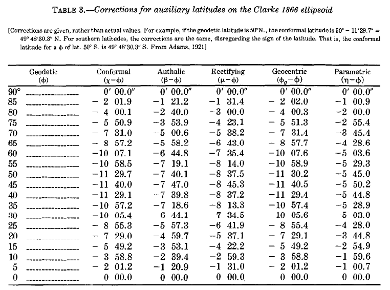
COMPUTATION OF SERIES #
Most of the trigonometric series approximations throughout this book (for example, equations (3-2) and (3-5)) are given in terms of multiple angles. In this arrangement, the coefficients converge to zero more rapidly, but handling by computer is normally somewhat slower than that occurring with nested trigonometric series. The latter are equivalent to power polynomials and require a minimum number of computations of trigonometric functions from series built into the software of most computers.
The pertinent series in this book fall into one of three forms (3-34), (3-36) and (3-38), in which $\phi$ may be any variable, and $f(\phi)$ is the function:
If:
These are exact equivalents of the series as shown. First the primed coefficients are computed once for the full set of conversions from the original coefficients of (3-34), (3-36), or (3-38), then $\sin{2\phi}$ and $\cos{2\phi}$ are computed once for each point in (3-35), or $\sin{\phi}$ and $\sin^2{\phi}$ once for each point in (3-37), or $\cos{2\phi}$ once for each point in (3-39). Computation of $f(\phi)$ may then proceed from the innermost nest outward with a speed up to 25-35 percent faster than that with multiple-angle series.
For more efficient transformation of a great number of points from one set of coordinates to another, polynomial approximations for the entire projection may be considered. This is normally only practical for a limited region. For techniques in determining the polynomial coefficients, the reader is referred to Snyder (1985a, p. 5-6, 15-24).