4. SCALE VARIATION AND ANGULAR DISTORTION #
Since no map projection maintains correct scale throughout, it is important to determine the extent to which it varies on a map. On a world map, qualitative distortion is evident to an eye familiar with maps, after noting the extent to which landmasses are improperly sized or out of shape, and the extent to which meridians and parallels do not intersect at right angles, or are not spaced uniformly along a given meridian or given parallel. On maps of countries or even of continents, distortion may not be evident to the eye, but it becomes apparent upon careful measurement and analysis.
TISSOT’S INDICATRIX #
In 1859 and 1881, Nicolas Auguste Tissot published a classic analysis of the distortion which occurs on a map projection (Tissot, 1881; Adams, 1919, p. 153-163; Maling, 1973, p. 64-67). The intersection of any two lines on the Earth is represented on the flat map with an intersection at the same or a different angle. At almost every point on the Earth, there is a right angle intersection of two lines in some direction (not necessarily a meridian and a parallel) which are also shown at right angles on the map. All the other intersections at that point on the Earth will not intersect at the same angle on the map, unless the map is conformal, at least at that point. The greatest deviation from the correct angle is called $\omega$, the maximum angular deformation. For a conformal map, $\omega$ is zero. (In some texts, $2\omega$ is used rather than $\omega$.)
Tissot showed this relationship graphically with a special ellipse of distortion called an indicatrix. An infinitely small circle on the Earth projects as an infinitely small, but perfect, ellipse on any map projection. If the projection is conformal, the ellipse is a circle, an ellipse of zero eccentricity. Otherwise, the ellipse has a major axis and minor axis which are directly related to the scale distortion and to the maximum angular deformation. FIGURE 3.— Tissot’s Indicatrix. An infinitely small circle on the Earth (A) appears as an ellipse on a typical map (B). On a conformal map, (B) is a circle of the same or of a different size.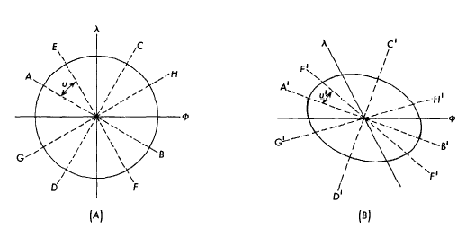
In figure 3, the left-hand drawing shows a circle representing the infinitely small circular element, crossed by a meridian $\lambda$ and parallel $\phi$ on the Earth. The right-hand drawing shows this same element as it may appear on a typical map projection. For general purposes, the map is assumed to be neither conformal nor equal-area. The meridian and parallel may no longer intersect at right angles, but there is a pair of axes which intersect at right angles on both Earth (AB and CD) and map (A’B’ and C’D’). There is also a pair of axes which intersect at right angles on the Earth (EF and GH), but at an angle on the map (E’F’ and G’H’) farthest from a right angle. The latter case has the maximum angular deformation $\omega$. The orientation of these axes is such that $\mu +\mu’ = 90° $, or, for small distortions, the lines fall about halfway between A’B’ and C’D’. The orientation is of much less interest than the size of the deformation. If $a$ and $b$, the major and minor semiaxes of the indicatrix, are known, then
Scale distortion is most often calculated as the ratio of the scale along the meridian or along the parallel at a given point to the scale at a standard point or along a standard line, which is made true to scale. These ratios are called “scale factors.” That along the meridian is called $h$ and along the parallel, $k$. The term “scale error” is frequently applied to $(h-1)$ and $(k-1)$. If the meridians and parallels intersect at right angles, coinciding with a and b in figure 3, the scale factor in any other direction at such a point will fall between $h$ and $k$. Angle $\omega$ may be calculated from equation (4-1), substituting $h$ and $k$ in place of $a$ and $b$. In general, however, the computation of $\omega$ is much more complicated, but is important for knowing the extent of the angular distortion throughout the map.
The formulas are given here to calculate $h$, $k$, and $\omega$ but the formulas for $h$ and $k$ are applied specifically to all projections for which they are deemed useful as the projection formulas are given later. Formulas for $\omega$ for specific projections have generally been omitted.
Another term occasionally used in practical map projection analysis is “convergence” or “grid declination.” This is the angle between true north and grid north (or direction of the Y axis). For regular cylindrical projections this is zero, for regular conic and polar azimuthal projections it is a simple function of longitude, and for other projections it may be determined from the projection formulas by calculus from the slope of the meridian $({\mathrm{d}x}/{\mathrm{d}y})$ at a given latitude. It is used primarily by surveyors for fieldwork with topographic maps. Convergence is not discussed further in this work.
DISTORTION FOR PROJECTIONS OF THE SPHERE #
The formulas for distortion are simplest when applied to regular cylindrical, conic (or conical), and polar azimuthal projections of the sphere. On each of these types of projections, scale is solely a function of the latitude.
Given the formulas for rectangular coordinates x and y of any cylindrical projection as functions solely of longitude $\lambda$ and latitude $\phi$, respectively,
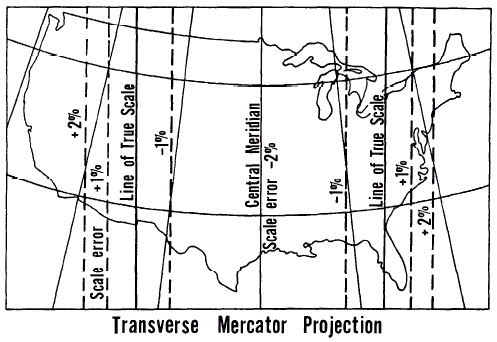
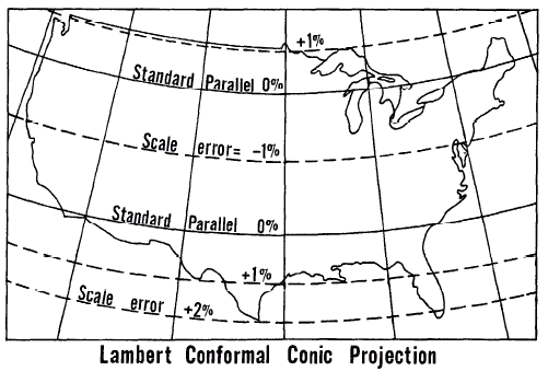
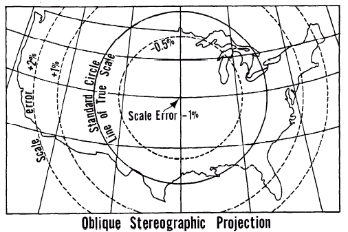
FIGURE 4.— Distortion patterns on common conformal map projections. The Transverse Mercator and the Stereographic are shown with reduction in scale along the central meridian or at the center of projection, respectively. If there is no reduction, there is a single line of true scale along the central meridian on the Transverse Mercator and only a point of true scale at the center of the Stereographic. The illustrations are conceptual rather than precise, since each base map projection is an identical conic.
Given the formulas for polar coordinates $\rho$ and $\theta$ of any polar azimuthal projection as functions solely of $\phi$ and $\lambda$, respectively, equations (4-4) and (4-5) apply, with $n$ equal to 1.0: $$ h = -\dd \rho/(R\dd\phi) \tag{4-4} $$
An analogous relationship applies to scale factors on oblique cylindrical and conic projections.
For any of the pairs of equations from (4-2) through (4-8), the maximum angular deformation $\omega$ at any given point is calculated simply, as stated above,
For the general case, including all map projections of the sphere, rectangular coordinates $x$ and $y$ are often both functions of both $\phi$ and $\lambda$, so they must be partially differentiated with respect to both $\phi$ and $\lambda$, holding $\lambda$ and $\phi$, respectively, constant. Then,
(1) $s = h k$ if meridians and parallels intersect at right angles ($\theta’ = 90°$);
(2) $h = k$ and $\omega = 0$ if the map is conformal;
(3) $h = 1/k$ on an equal-area map if meridians and parallels intersect at right angles.1
DISTORTION FOR PROJECTIONS OF THE ELLIPSOID #
The derivation of the above formulas for the sphere utilizes the basic formulas for the length of a given spacing (usually 1° or 1 radian) along a given meridian or a given parallel. The following formulas give the length of a radian of latitude ($L_\phi$) and of longitude ($L_\lambda$) for the sphere:
The radius of curvature on a sphere is the same in all directions. On the ellipsoid, the radius of curvature varies at each point and in each direction along a given meridian, except at the poles. The radius of curvature $R’$ in the plane of the meridian is calculated as follows:
The length of a radian of latitude is defined as the circumference of a circle of this radius, divided by $2\pi$, or the radius itself. Thus,
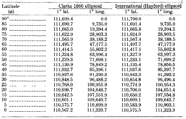
TABLE 4.— Lengths, in meters, of 1° of latitude and longitude on two ellipsoids of reference
For cylindrical projections:
For polar azimuthal projections:
Except for $C_s$ which is independent of $R/a$, $R$ must be given an arbitrary value such as $R_q$ (see equation (3-13)), $R_M$ (see second sentence following equation (3-22)), or another reasonable balance between the major and minor semiaxes $a$ and $b$ of the ellipsoid. Using $R_q$ and the Clarke 1866 ellipsoid, table 5 shows the magnitude of these corrections.
TABLE 5.— Ellipsoidal correction factors to apply to spherical projections based on Clarke 1866 ellipsoid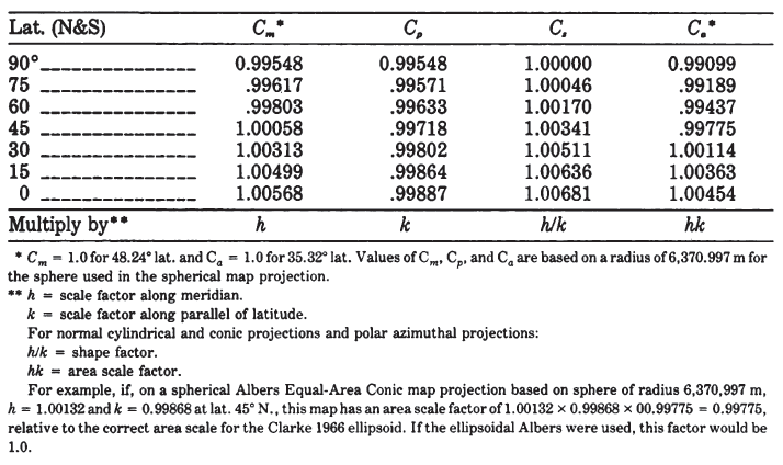
A map extending over a large area will have a scale variation of several percent, which far outweighs the significance of the less-than-1-percent variation between sphere and ellipsoid. A map of a small area, such as a large-scale detailed topographic map, or even a narrow strip map, has a small-enough intrinsic scale variation to make the ellipsoidal correction a significant factor in accurate mapping; e.g., a 7.5-min quadrangle normally has an intrinsic scale variation of 0.0002 percent or less.
CAUCHY-RIEMANN AND RELATED EQUATIONS #
Relatively simple equations provide necessary and sufficient conditions for any map projection, spherical or ellipsoidal, to be conformal. These are called the Cauchy-Riemann equations after two 19th-century mathematicians. The concept had been devised, however, during the 18th century. These equations may be written as follows:
Analogous relationships may be obtained for equal-area transformations. The following equation applies to the ellipsoid:
An equal-area transformation from one set of rectangular coordinates to another must satisfy the following relationship:
Most of the above equations (4-33) through (4-44) are difficult to use to derive new projections, although they may be used to determine whether existing projections are conformal or equal-area. Equation (4-43), however, may be fairly readily used to devise new projections which are pseudocylindrical and equal-area. Equation (26-4), discussed later, is a general equation satisfying (4-39) and (4-40), although it is not the only such equation. There is no known general equation satisfying equation (4-44) except in a very elementary way.