5. TRANSFORMATION OF MAP GRATICULES #

As discussed later, several map projections have been adapted to showing some part of the Earth for which the lines of true scale have an orientation or location different from that intended by the inventor of the basic projection. This is equivalent to moving or transforming the graticule of meridians and parallels on the Earth so that the “north pole” of the graticule assumes a position different from that of the true North Pole of the Earth. The projection for the sphere may be plotted using the original formulas or graphical construction, but applying them to the new graticule orientation. The actual meridians and parallels may then be plotted by noting their relationship on the sphere to the new graticule, and landforms drawn with respect to the actual geographical coordinates as usual.

In effect, this procedure was used in the past in an often entirely graphical manner. It required considerable care to avoid cumulative errors resulting from the double plotting of graticules. With computers and programmable hand calculators, it now can be a relatively routine matter to calculate directly the rectangular coordinates of the actual graticule in the transformed positions or, with an automatic plotter, to obtain the transformed map directly from the computer.

The transformation most notably has been applied to the azimuthal and cylindrical projections, but in a few cases it has been used with conic, pseudocylindrical, and other projections. While it is fairly straightforward to apply a suitable transformation to the sphere, transformation is much more difficult on the ellipsoid because of the constantly changing curvature. Transformation has been applied to the ellipsoid, however, in important cases under certain limiting conditions. If either true pole is at the center of an azimuthal map projection, the projection is called the polar aspect. If a point on the Equator is made the center, the projection is called the equatorial or, less often, meridian or meridional aspect. If some other point is central, the projection is the oblique or, occasionally, horizon aspect.

For cylindrical and most other projections, such transformations are called transverse or oblique, depending on the angle of rotation. In transverse projections, the true poles of the Earth lie on the equator of the basic projection, and the poles of the projection lie on the Equator of the Earth. Therefore, one meridian of the true Earth lies along the equator of the basic projection. The Transverse Mercator projection is the best-known example and is related to the regular Mercator in this manner. For oblique cylindrical projections, the true poles of the Earth lie somewhere between the poles and the equator of the basic projection. Stated another way, the equator of the basic projection is drawn along some great circle route other than the Equator or a meridian of the Earth for the oblique cylindrical aspect. The Oblique Mercator is the most common example. Further subdivisions of these aspects have been made; for example, the transverse aspect may be first transverse, second transverse, or transverse oblique, depending on the positions of the true poles along the equator of the basic projection (Wray, 1974). This has no significance in a transverse cylindrical projection, since the appearance of the map does not change, but for pseudocylindrical projections such as the Sinusoidal, it makes a difference, if the additional nomenclature is desired.

To determine formulas for the transformation of the sphere, two basic laws of spherical trigonometry are used. Referring to the spherical triangle in figure 5, with three points having angles $A$, $B$, and $C$ on the sphere, and three great circle arcs $a$, $b$, and $c$ connecting them, the Law of Sines declares that

$$ \sin A/\sin a = \sin B/\sin b = \sin C/\sin c \tag{ 5-1 } $$

while by the Law of Cosines,

$$ \cos c = \cos b \cos a + \sin b \sin a \sin C \tag{ 5-2 } $$

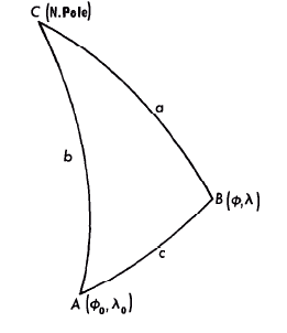
FIGURE 5.— Spherical triangle. — **FIGURE 5**.— Spherical triangle.

If C is placed at the North Pole, it becomes the angle between two meridians extending to A and B. If A is taken as the starting point on the sphere, and B the second point, c is the great circle distance between them, and angle A is the azimuth Az east of north which point B bears to point A. When latitude ϕ₁, and longitude λ₀, are used for point A, and ϕ and λ are used for point B, equation (5-2) becomes the following for great circle distance:

$$ \cos c = \sin\phi_1\sin\phi + \cos\phi_1\cos\phi\cos{(\lambda-\lambda_0)} \tag{ 5-3 } $$

While (5-3) is the standard and simplest form of this equation, it is not accurate in practical computation for values of c very close to zero. For such cases, the equation may be rearranged as follows (Sinnott, 1984):

$$ \sin(c/2)=|\sin^2[(\phi-\phi_1)/2] + \cos\phi_1\cos\phi\cos(\lambda-\lambda_0)|^{1/2} \tag{ 5-3a } $$

This equation is also exact, and is very accurate in practice for values of c from 0 to nearly 180°.

Equation (5-1) becomes the following for the azimuth:

$$ \sin{Az} = \sin(\lambda-\lambda_0)\cos\phi/\sin c \tag{ 5-4 } $$

or, with some rearrangement,

$$ \cos{Az} = [cos\phi_1\sin\phi - \sin\phi_1\cos\phi\cos(\lambda-\lambda_0)]/\sin c \tag{ 5-4a } $$

or, eliminating c,

$$ \tan{Az} = \cos\phi\sin(\lambda-\lambda_0)/[\cos\phi_1\sin\phi - \sin\phi_1\cos\phi\cos(\lambda-\lambda_0)] \tag{ 5-4b } $$

Either of the three equations (5-4) through (5-4b) may be used for the azimuth, depending on the form of equation preferred. Equation (5-4b) is usually preferred, since it avoids the inaccuracies of finding an arcsin near 90° or an arccos near 0°. Quadrant adjustment as described under the list of symbols should be employed.

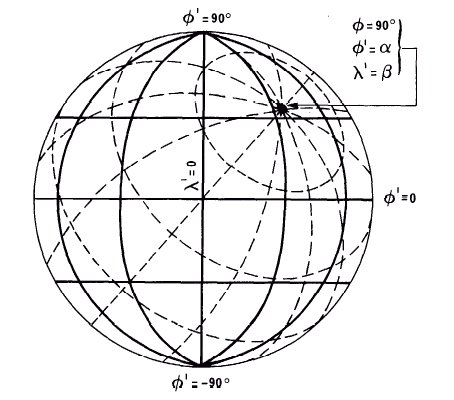
FIGURE 6.— Rotation of a graticule for transformation of projection. Dashed lines show actual longitudes and latitudes (λ and ϕ). Solid lines show the transformed longitudes and latitudes (λ’ and ϕ’) from which rectangular coordinates (x and y) are determined according to map projection used. — **FIGURE 6**.— Rotation of a graticule for transformation of projection. Dashed lines show actual longitudes and latitudes (λ and ϕ). Solid lines show the transformed longitudes and latitudes (λ’ and ϕ’) from which rectangular coordinates (x and y) are determined according to map projection used.

In order to find the latitude $\phi$ and longitude $\lambda$ at a given arc distance $c$ and azimuth $Az$ east of north from $(\phi_1, \lambda_0)$, the inverse of equations (5-3) and (5-4b) may be used:

$$ \phi = \arcsin(\sin\phi_1\cos c + \cos\phi_1\cos{Az}) \tag{ 5-5 } $$

$$ \lambda = \lambda_0 + \arctan[\sin c \, \sin{Az}/(\cos\phi_1\cos c - \sin\phi_1\sin c\,\cos{Az})] \tag{ 5-6 } $$

Applying these relationships to transformations, without showing some intermediate derivations, formulas (5-7) through (5-8b) are obtained. To place the North Pole of the sphere at a latitude $\alpha$ on a meridian $\beta$ east of the central meridian $(\lambda’=0)$ of the basic projection (see fig. 6), the transformed latitude $\phi’$ and transformed longitude $\lambda’$ on the basic projection which correspond to latitude $\phi$ and longitude $\lambda$ of the spherical Earth may be calculated as follows, letting the central meridian to correspond with $\lambda’ = \beta$:

$$ \sin\phi' = \sin\alpha\sin\beta - \cos\alpha\cos\phi\cos(\lambda-\lambda_0) \tag{ 5-7 } $$

$$ \sin(\lambda'-\beta) = cos\phi\sin(\lambda-\lambda_0)/\cos\phi' \tag{ 5-8 } $$

Equation (5-8b) is generally preferable to (5-8) or (5-8a) for the reasons stated after equation (5-4b).

These are general formulas for the oblique transformation. (For azimuthal projections, $\beta$ may always be taken as zero. Other values of $\beta$ merely have the effect of rotating the X and Y axes without changing the projection.)

The inverse forms of these equations are similar in appearance. To find the geographic coordinates in terms of the transformed coordinates,

$$ \sin\phi = \sin\alpha\sin\phi' + \cos\alpha\cos\phi'\cos(\lambda'-\beta) \tag{ 5-9 } $$

$$ \sin(\lambda-\lambda_0) = \cos\phi'\sin(\lambda'-\beta)/\cos\phi \tag{ 5-10 } $$

$$ \cos(\lambda-\lambda_0) = [\sin\alpha\cos\phi'\cos(\lambda'-\beta) - \cos\alpha\,\sin\phi']/\cos\phi \tag{ 5-10a } $$

$$ \tan(\lambda-\lambda_0) = \cos\phi'\sin(\lambda'-\beta)/[\sin\alpha\,\cos\phi'\cos(\lambda'-\beta) - \cos\alpha\,\sin\phi'] \tag{ 5-10b } $$

with equation (5-10b) usually preferable to (5-10) and (5-10a) for the same reasons as those given for (5-4b).

If $\alpha = 0$, the formulas simplify considerably for the transverse or equatorial aspects. It is then more convenient to have central meridian$\lambda_0$, coincide with the equator of the basic projection rather than with its meridian $\beta$. This may be accomplished by replacing $(\lambda-\lambda_0)$ with $(\lambda-\lambda_0 -90°)$ and simplifying. If $\beta = 0$, so that the true North Pole is placed at $(\lambda_0 = 0,\> \phi’ = 0)$:

$$ \sin\phi' = -\cos\phi\sin(\lambda-\lambda_0) \tag{ 5-11 } $$

$$ \cos\lambda' = \sin\phi/[1-\cos^2\phi\sin^2(\lambda-\lambda_0)]^{1/2} \tag{ 5-12 } $$

$$ \tan\lambda' = -\cos(\lambda-\lambda_0)/\tan\phi \tag{ 5-12a } $$

If $\beta=90°$, placing the true North Pole at $(\lambda’=90°, \> \phi’ = 0)$:

$$ \sin\phi' = -\cos\phi\sin(\lambda-\lambda_0) \tag{ 5-13 } $$

$$ \cos\lambda' = \cos\phi\cos(\lambda-\lambda_0)/[1-\cos^2\phi\sin^2(\lambda-\lambda_0)]^{1/2} \tag{ 5-14 } $$

$$ \tan\lambda' = \tan\phi/\cos(\lambda-\lambda_0) \tag{ 5-14a } $$

The inverse equations (5-9) through (5-10b) may be similarly altered. As stated earlier, these formulas may be directly incorporated into the formulas for the rectangular coordinates x and y of the basic map projection for a direct computer or calculator output. If only one or two projections are involved in a package, this may be more efficient. For such transformations of several projections in one software package, it is often easier to calculate the transverse or oblique projection coordinates by first calculating $\phi’$ and $\lambda’$ for each point to be plotted (using a general subroutine) and then calculating the rectangular coordinates by inserting $\phi’$ and $\lambda’$ into the basic projection formulas In still other cases, a graphical method has been used.

While these formulas, or their equivalents, will be incorporated into the formulas given later for individual oblique and transverse projections, the concept should help interrelate the various aspects or types of centers of a given projection. The extension of these concepts to the ellipsoid is much more involved technically and in some cases requires approximation. General discussion of this is omitted here.