10. CYLINDRICAL EQUAL-AREA PROJECTION #

SUMMARY #

• Cylindrical.
• Equal-area.
• Meridians on normal aspect are equally spaced straight lines.
• Parallels on normal aspect are unequally spaced straight lines, closest near the poles, cutting meridians at right angles.
• On transverse aspect, central meridian, each meridian 90° from central meridian, and Equator are straight lines. Other meridians and parallels are complex curves.
• On oblique aspect, two meridians 180° apart are straight lines. Other meridians and parallels are complex curves.
• On normal aspect, scale is true along Equator, or along two parallels equidistant from the Equator.
• On transverse aspect, scale is true along central meridian, or along two straight lines equidistant from and parallel to central meridian. (These lines are only approximately straight for the ellipsoid.)
• On oblique aspect, scale is true along chosen central line, an oblique great circle, or along two straight lines parallel to central line. Scale on ellipsoidal form is similar, but varies slightly from this pattern.
• An orthographic projection of sphere onto cylinder.
• Substantial shape and scale distortion near points 90° from central line.
• Normal and transverse aspects presented by Lambert in 1772.

HISTORY AND USAGE #

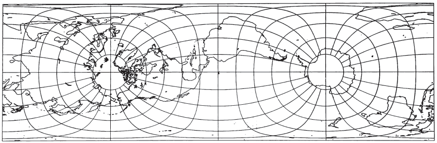
The fourth of the seven projections proposed by Johann Heinrich Lambert (1772, p. 71-72) and occasionally given his name, is the Cylindrical Equal-Area (fig. 14). In the same work (p. 72-73), he described its transverse aspect (fig. 16), which has hardly been used. Even the normal aspect has seldom been used except as a textbook example of the most easily constructed equal-area projection, but several modifications of the normal aspect have been published.

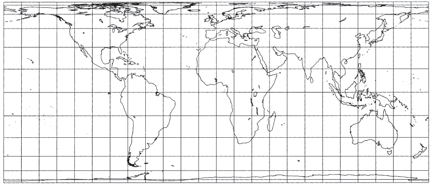
These modifications consist of compressing the projection from east to west and expanding it in the same ratio from north to south, thereby moving the parallel of no distortion from the Equator to other latitudes. The earliest such modification is from Scotland: James Gall’s Orthographic Cylindrical, not the same as his preferred Stereographic Cylindrical, both of which were originated in 1855, has standard parallels of 45° N. and S. (Gall, 1885). Walther Behrmann (1910) of Germany chose 30°, based on certain overall distortion criteria (fig. 15). Very similar later projections were offered by Trystan Edwards of England in 1953 and Arno Peters of Germany in 1967; they were presented as revolutionary and original concepts, rather than as modifications of these prior projections with standard parallels at about 37° and 45°-47°, respectively (Maling, 1966, 1974).

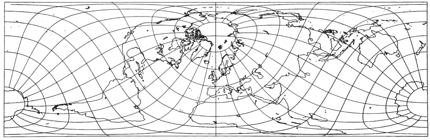
The oblique Cylindrical Equal-Area projection has been proposed with particular parameters for maps of Eurasia and Africa (Thornthwaite, 1927) and of air routes of the British Commonwealth (Poole, 1934). Different parameters are used for fig. 17. The ellipsoidal form of the oblique and transverse aspects has apparently been developed only recently (Snyder, 1985b).

FEATURES #

Like other regular cylindricals, the graticule of the normal Cylindrical Equal-Area projection consists of straight equally spaced vertical meridians perpendicular to straight unequally spaced horizontal parallels. To achieve equality of area, the parallels are spaced from the Equator in proportion to the sine of the latitude. This is the simplest equal-area projection.

The normal Cylindrical Equal-Area for the sphere is a true perspective projection onto a cylinder tangent at the Equator: The meridians are projected from the center of the sphere, and the parallels are projected with lines parallel to the equatorial plane, or orthographically from infinity. Modifications such as Behrmann’s, described above, are perspective projections onto a secant cylinder. For oblique and transverse aspects, the projection may be perspectively cast on a cylinder tangent or secant at an oblique angle, or centered on a meridian.

There is no distortion of area anywhere on the projections, and no distortion of scale and shape at the standard parallels of the normal aspect, or at the standard lines of the oblique or transverse aspects. There is extreme shape and scale distortion 90° from the central line, or at the poles on the normal aspect. These are the points which have infinite area and linear scale on the various aspects of the Mercator projection. This distortion, even on the modifications described above, is so great that there has been little use of any of the forms for world maps by professional cartographers, and many of them have strongly criticized the intensive promotion in the noncartographic community which has accompanied the presentation of one of the recent modifications.

The meridians and parallels of the transverse and oblique aspects which are straight or curved on the Mercator projection are straight or curved, respectively, on the Cylindrical Equal-Area, except that the curves are differently shaped.

In spite of the shape distortion in some portions of a world map, the projection is well suited for equal-area mapping of regions which are predominantly north-south in extent, or which have an oblique central line, or which lie near the Equator. This is true in the same sense that for mid-latitude regions which extend predominantly east-west, the Albers Equal-Area Conic projection is recommended for equal-area mapping. Actually, the normal Cylindrical Equal-Area is the limiting form of the Albers when the Equator or two parallels symmetrical about the Equator are made standard. If such regions to be mapped are smaller than the United States, the ellipsoidal form should be considered.

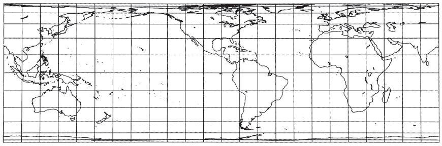
FORMULAS FOR THE SPHERE #

The geometric construction of the Cylindrical Equal-Area projection has been described above. The forward formulas for the normal aspect are as follows, given $R, \phi_s,\lambda_0$, \phi and $\lambda$ to find $x$ and $y$ (see numerical examples):

For the oblique aspect, the alternatives used for the Oblique Mercator projection are used here, with modification only in the formulas for the $y$ coordinates:

1. Given two points to lie upon the central line, with latitudes and longitudes $(\phi_1, \lambda_1)$ and $(\phi_2, \lambda_2)$, and longitude increasing easterly and relative to Greenwich, the pole of the oblique transformation at $(\phi_p, \lambda_p)$ may be calculated as follows:

   $$ \begin{align} \lambda_p = &\arctan[(\cos\phi_1\sin\phi_2\cos\lambda_1 - \sin\phi_1\cos\phi_2\cos\lambda_2)/ \\ &(\sin\phi_1\cos\phi_2\sin\lambda_2 - \cos\phi_1\sin\phi_2\sin\lambda_1)] \end{align} \tag{ 9-1 } $$
   $$ \phi_p = \arctan[-\cos(\lambda_p-\lambda_1)/\tan\phi_1] \tag{ 9-2 } $$
   The Fortran ATAN2 function or its equivalent should be used with equation (9-1), but not with (9-2). The other pole is located at $(-\phi_p,\lambda_p\pm\pi)$. Using the positive (northern) value of $\phi_p$, the following formulas give the rectangular coordinates for point $(\phi,\lambda)$, with $h_0$, the scale factor along the central line:
   $$ x= Rh_0\arctan\{[\tan\phi\cos\phi_p+\sin\phi_p\sin(\lambda-\lambda_0)]/\cos(\lambda-\lambda_0)\} \tag{ 10-4 } $$
   $$ y= (R/h_0)[\sin\phi_p\sin\phi-\cos\phi_p\cos\phi\sin(\lambda-\lambda_0)] \tag{ 10-5 } $$
   With these formulas for the oblique aspect, the origin of rectangular coordinates lies at
   $$ \eqalign{ \phi_0 &= 0 \cr \lambda_0 &=\phi_p + \pi/2 } \tag{ 9-6a } $$
   and the X axis lies along the central line, $x$ increasing easterly. The transformed poles are straight lines at $y = R$ and are as long as the central line.

2. Given a central point $(\phi_z,\lambda_z)$ with longitude increasing easterly and relative to Greenwich, and azimuth $\gamma$ east of north of the central line through $(\phi_z,\lambda_z)$, the pole of the oblique transformation at $(\phi_p,\lambda_p)$ may be calculated as follows:

   $$ \phi_p = \arcsin(\cos\phi_z\sin\gamma) \tag{ 9-7 } $$
   $$ \lambda_p = \arctan[-\cos\beta(-\sin\phi_z\sin\gamma)]+ \lambda_z \tag{ 9-8 } $$
   These values of $\phi_p$ and $\lambda_p$, may then be used in equations (10-4) and (10-5) as before.

For the inverse formulas, first for the normal aspect, given $R, \phi_s, \lambda_0, x,$ and $y$, to find $\phi$ and $\lambda$:

For the oblique aspect, equations (9-1) and (9-2) or (9-7) and (9-8) must first be used to establish the pole of the oblique transformation, if it is not known already. Then

FORMULAS FOR THE ELLIPSOID #

In the following formulas, the ellipsoid is transformed onto the authalic sphere, but the scale along the desired central line is made constant by variably compressing the scale along this central line to match that along the same path on the ellipsoid. To retain correct area, the distances perpendicular to the central line are increased by the same ratio. For the oblique aspect, the central line is not a geodesic, but is instead an oblique great circle on the authalic sphere.

For the forward formulas using the normal aspect, given $a, e, \phi_s, \lambda_0, \phi$, and $\lambda$, to find $x$ and $y$ (see numerical examples), the equations are given in the order of computation:

For the transverse aspect, the subsequent formulas for the oblique aspect may be used, but the following are simpler for the transverse alone. Given $a, e, h_0, \lambda_0, \phi_0, \phi,$ and $\lambda$, to find $x$ and $y$, first $q$ is calculated from $\phi$ using equation (3-12) above. Then

For the oblique aspect, the location of the pole $(\phi_p,\lambda_p)$ may be given, or it may be computed as described under the section on formulas for the sphere above. Points $\phi_1, \phi_2, \phi_p$ and $\phi_z$, however, are replaced in equations (9-1), (9-2), (9-7) and (9-8) with $\beta_1, \beta_2, \beta_p$ and $\beta_z$ respectively, and $\beta_p$ is finally converted to $\phi_p$, using equations (10-17) and (3-16), or just (3-18), and subscripts $p$ instead of $c$.

If the ellipsoid is either the Clarke 1866 or the International, Fourier constants may be taken from table 13.

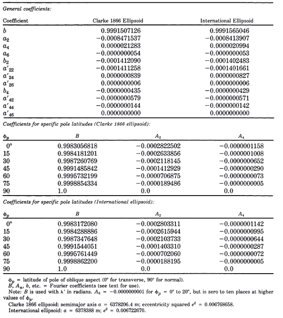
For the inverse formulas for the ellipsoid, the normal aspect will be discussed first. Given $a, e, \phi_s,\lambda_0, x$, and $y$, to find $\phi$ and $\lambda$ (see p. 284 for numerical examples), $k_0$ is determined from (10-13), and

For the transverse aspect, given $a, e, h_0, \lambda_0, x$, and $y$, to find $\phi$ and $\lambda$:

For the oblique aspect, given $a, e, h_0, \phi_p, \lambda_p, x$, and $y$, to find $\phi$ and $\lambda$, Fourier coefficients are determined as described above for the forward oblique ellipsoidal formulas, while the pole location $(\phi_p,\lambda_p)$, may be determined if not provided, as described for the forward oblique spherical formulas, and $q_p$ is found from (3-12) using 90° for $\phi$. From $x, \lambda’$ is determined from an iterative inverse of (10-23):

Equation (10-24) above is used to find $F$ from $\lambda’$. Then,

For the determination of Fourier coefficients, if they are not already provided, equation (10-23) above is equivalent to the following equation which requires numerical integration:

To compute $F$ from equation (10-37) for a given $\lambda’$, first $\beta_p$ is found from $\phi_p$ using (3-12) and (3-11), subscripting $\phi$ and $\lambda$ with p. Then,