11. MILLER CYLINDRICAL PROJECTION #
SUMMARY #
- Neither equal-area nor conformal.
- Used only in spherical form.
- Cylindrical.
- Meridians and parallels are straight lines, intersecting at right angles.
- Meridians are equidistant; parallels spaced farther apart away from Equator.
- Poles shown as lines.
- Compromise between Mercator and other cylindrical projections.
- Used for world maps.
- Presented by Miller in 1942.
HISTORY AND FEATURES #
The need for a world map which avoids some of the scale exaggeration of the Mercator projection has led to some commonly used cylindrical modifications, as well as to other modifications which are not cylindrical. The earliest common cylindrical example was developed by James Gall of Edinburgh about 1855 (Gall, 1885, p. 119-123). His meridians are equally spaced, but the parallels are spaced at increasing intervals away from the Equator. The parallels of latitude are actually projected onto a cylinder wrapped about the sphere, but cutting it at lats. 45° N. and S., the point of perspective being a point on the Equator opposite the meridian being projected. It is used in several British atlases, but seldom in the United States. The Gall projection is neither conformal nor equal-area, but has a blend of various features. Unlike the Mercator, the Gall shows the poles as lines running across the top and bottom of the map.
What might be called the American version of the Gall projection is the Miller Cylindrical projection (fig. 18), presented in 1942 by Osborn Maitland Miller (1897-1979) of the American Geographical Society, New York (Miller, 1942). Born in Perth, Scotland, and educated in Scotland and England, Miller came to the Society in 1922. There he developed several improved surveying and mapping techniques. An expert in aerial photography, he developed techniques for converting high-altitude photographs into maps. He led or joined several expeditions of explorers and advised leaders of others. He retired in 1968, having been best known to cartographers for several map projections, including the Bipolar Oblique Conic Conformal, the Oblated Stereographic, and especially his Cylindrical projection.
Miller had been asked by S. Whittemore Boggs, Geographer of the U.S. Department of State, to study further alternatives to the Mercator, the Gall, and other cylindrical world maps. In his presentation, Miller listed four proposals, but the one he preferred, and the one used, is a fairly simple mathematical modification of the Mercator projection. Like the Gall, it shows visible straight lines for the poles, increasingly spaced parallels away from the Equator, equidistant meridians, and is not equal-area, equidistant along meridians, nor conformal. While the standard parallels, or lines true to scale and free of distortion, on the Gall are at lats. 45° N. and S., on the Miller only the Equator is standard. Unlike the Gall, the Miller is not a perspective projection.
The Miller Cylindrical projection is used for world maps and in several atlases, including the National Atlas of the United States (USGS, 1970, p. 330-331). As Miller (1942) stated,
the practical problem considered here is to find a system of spacing the parallels of latitude such that an acceptable balance is reached between shape and area distortion. By an “acceptable” balance is meant one which to the uncritical eye does not obviously depart from the familiar shapes of the land areas as depicted by the Mercator projection but which reduces areal distortion as far as possible under these conditions * * *. After some experimenting, the [Modified Mercator (b)] was judged to be the most suitable for Mr. Boggs’s purpose * * *.
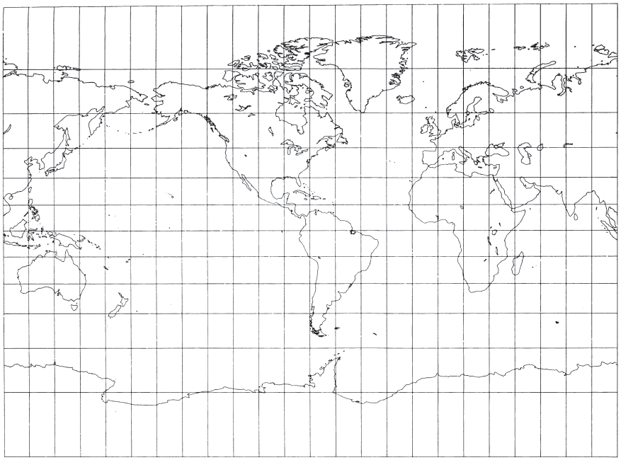
FIGURE 18.— The Miller Cylindrical Projection. A projection resembling the Mercator, but having less relative distortion in polar regions. Neither conformal nor equal-area.
FORMULAS FOR THE SPHERE #
Miller’s spacings of parallels from the Equator are the same as if the Mercator spacings were calculated for 0.8 times the respective latitudes, with the result divided by 0.8. As a result, the spacing of parallels near the Equator is very close to the Mercator arrangement.
The forward formulas, then, are as follows (see numerical example):
The inverse equations are easily derived from equations (11-1) through (11-2a):
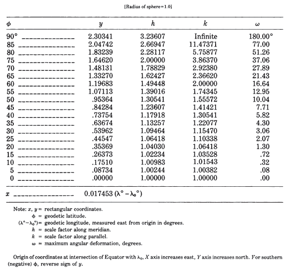
Rectangular coordinates are given in table 14. There is no basis for an ellipsoidal equivalent, since the projection is used for maps of the entire Earth and not for local areas at large scale. TABLE 14.— Miller Cylindrical projection: Rectangular coordinates