13. CASSINI PROJECTION #
SUMMARY #
- Cylindrical.
- Neither equal-area nor conformal.
- Central meridian, each meridian 90" from central meridian, and Equator are straight lines.
- Other meridians and parallels are complex curves.
- Scale is true along central meridian, and along lines perpendicular to central
- meridian. Scale is constant but not true along lines parallel to central meridian on spherical form, nearly so for ellipsoid.
- Used for topographic mapping formerly in England and currently in a few other countries.
- Devised by C. F. Cassini de Thury in 1745 for the survey of France.
HISTORY #
Although the Cassini projection has been largely replaced by the Transverse Mercator, it is still in limited use outside the United States and was one of the major topographic mapping projections until the early 20th century. It was first developed by César François Cassini de Thury (1714-1784), grandson of Jean Dominique Cassini. The latter was an outstanding Italian-born astronomer who changed his given names from Giovanni Domenico after being hired in 1669 for astronomical research in Paris, and soon thereafter to begin the survey of France. Cassini de Thury was the third of four generations involved in this project, the first detailed survey of a nation. In 1745 he devised the projection which, with some modifications, still bears the family name and was used for official topographic maps of France until its replacement by the Bonne projection in 1803.
Instead of showing meridians and parallels (except for the central meridian), Cassini employed a system of squares with rectangular grid coordinates, the meridian through Paris serving as one axis. The scale along this central meridian was made correct according to the surveyed distance, thus approximately correcting for the ellipsoid (Craig, 1882, p. 80; Reignier, 1957, p. 98-99). Mathematical analysis by J. G. von Soldner in the early 19th century led to more accurate ellipsoidal formulas, and the name Cassini-Soldner is often used for the form used in topographic mapping.
FEATURES #
The spherical form of the Cassini projection (fig. 19) bears the same relation to the Equidistant Cylindrical or Plate Carrée projection that the spherical Transverse Mercator bears to the regular Mercator. Instead of having the straight meridians and parallels of the Equidistant Cylindrical, the Cassini has complex curves for each, except for the Equator, the central meridian, and each meridian 90° away from the central meridian, all of which are straight. FIGURE 19.— Cassini projection. A transverse Equidistant Cylindrical projection used for large-scale mapping in France, England, and several other countries. Largely replaced by conformal mapping.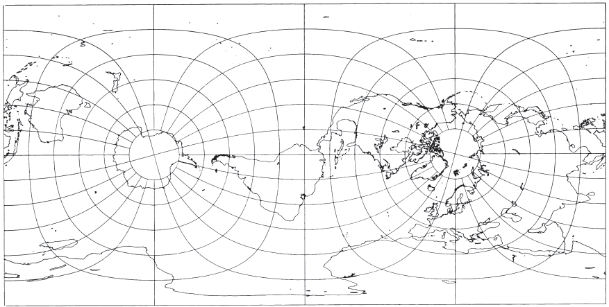
By making a given point (such as Washington, D.C.) the pole on an oblique Equidistant Cylindrical projection, the bearing and distance from that point to any other on the Earth can be read directly as two rectangular coordinates (Botley, 1951). This provides the same information as the oblique Azimuthal Equidistant projection centered on the same point. The oblique cylindrical has the advantage of offering rectangular instead of polar coordinates, but the map is much more distorted near the chosen point.
The scale is correct along the central meridian and also along any straight line perpendicular to the central meridian. It gradually increases in a direction parallel to the central meridian, as the distance from that meridian increases, but the scale is constant along any straight line on the map which is parallel to the central meridian. Therefore, the Cassini is more suitable for regions predominantly north-south in extent, such as Great Britain, than for regions extending in other directions. In this respect, it is also like the Transverse Mercator. The projection is neither equal-area nor conformal, but it has a compromise of both features.
The ellipsoidal form is computed from series which are essentially modifications of those for the ellipsoidal form of the Transverse Mercator and are suitable within only a few degrees to either side of the central meridian. The scale characteristics described above for the spherical form apply to the ellipsoidal form, except that the lines of constant scale paralleling the central meridian are not quite straight.
USAGE #
There has been little usage of the spherical version of the Cassini, but the ellipsoidal Cassini-Soldner version was adopted by the Ordnance Survey for the official survey of Great Britain during the second half of the 19th century (Steers, 1970, p. 229). Many of these maps were prepared at a scale of 1:2,600. The Cassini-Soldner was also used for the detailed mapping of many German states during the same period.
Beginning about 1920, the Ordnance Survey began to change to the Transverse Mercator because of the difficulty of measuring scale and direction on the Cassini. Nevertheless, there are several maps still in print which are based on the older projection in Great Britain, and the projection is used in a few other countries such as Cyprus, Czechoslovakia, Denmark, the Federal Republic of Germany, and Malaysia (Clifford J. Mugnier, personal comm., 1985).
A system equivalent to an oblique Equidistant Cylindrical or oblique Cassini projection was used in early coordinate transformations for ERTS (now Landsat) satellite imagery, but it was changed in 1978 to the Hotine Oblique Mercator, and in 1982 to the Space Oblique Mercator projection.
FORMULAS FOR THE SPHERE #
For the forward formulas, given $R, \phi_o, \lambda_0, \phi$, and $\lambda$, to find $x$ and $y$:
The inverse formulas for $(\phi,\lambda)$ in terms of $(x, y)$:
FORMULAS FOR THE ELLIPSOID #
For the ellipsoidal form, a set of series approximations is given for use in a zone extending 3° to 4° of longitude from the central meridian. Coordinate axes are the same as they are for the spherical formulas above. The formulas below are adapted from those provided by Clifford J. Mugnier (pers. commun., 1979; see also Clark and Clendinning, 1944).
$M_0 = M$ calculated for $\phi_0$, the latitude crossing the central meridian $\lambda_0$ at the origin of the $x, y$ coordinates. The choice of $\phi_0$ does not affect the shape of the projection.
$s =$ the scale factor at an azimuth $Az$ east of north for a given $\phi$ and $x$.
From $\phi_1$, other terms below are calculated for use in equations (13-10) and (13-11). (If $\phi_1=\pm\pi/2, \thinspace \phi=\pm90^\circ$, taking the sign of $y$, while $\lambda$ is indeterminate, and may be called $\lambda_0$.)