7. MERCATOR PROJECTION #

SUMMARY #

Cylindrical.
Conformal.
Meridians are equally spaced straight lines.
Parallels are unequally spaced straight lines, closest near the Equator, cutting meridians at right angles.
Scale is true along the Equator, or along two parallels equidistant from the Equator.
Loxodromes (rhumb lines) are straight lines.
Not perspective.
Poles are at infinity; great distortion of area in polar regions.
Used for navigation.
Presented by Mercator in 1569.

HISTORY #

The well-known Mercator projection was perhaps the first projection to be regularly identified when atlases of over a century ago gradually began to name projections used, a practice now fairly commonplace. While the projection was apparently used by Erhard Etzlaub (1462-1532) of Nuremberg on a small map on the cover of some sundials constructed in 1511 and 1513, the principle remained obscure until Gerardus Mercator (1512-94) (fig. 7) independently developed it and presented it in 1569 on a large world map of 21 sections totaling about 1.3 by 2 m (Keuning, 1955, p. 17-18).

Mercator, born at Rupelmonde in Flanders, was probably originally named Gerhard Cremer (or Kremer), but he always used the latinized form. To his contemporaries and to later scholars, he is better known for his skills in map and globe making, for being the first to use the term “atlas” to describe a collection of maps in a volume, for his calligraphy, and for first naming North America as such on a map in 1538. To the world at large, his name is identified chiefly with his projection, which he specifically developed to aid navigation. His 1569 map is entitled “Nova et Aucta Orbis Terrae Descriptio ad Usum Navigantium Emendate Accommodata (A new and enlarged description of the Earth with corrections for use in navigation).” He described in Latin the nature of the projection in a large panel covering much of his portrayal of North America:

In this mapping of the world we have [desired] to spread out the surface of the globe into a plane that the places shall everywhere be properly located, not only with respect to their true direction and distance, one from another, but also in accordance with their due longitude and latitude; and further, that the shape of the lands, as they appear on the globe, shall be preserved as far as possible. For this there was needed a new arrangement and placing of meridians, so that they shall become parallels, for the maps hitherto produced by geographers are, on account of the curving and the bending of the meridians, unsuitable for navigation. Taking all this into consideration, we have somewhat increased the degrees of latitude toward each pole, in proportion to the increase of the parallels beyond the ratio they really have to the equator. (Fite and Freeman, 1926, p. 77-78.)

Mercator probably determined the spacing graphically, since tables of secants had not been invented. Edward Wright (ca. 1558-1615) of England later developed the mathematics of the projection and in 1599 published tables of cumulative secants, thereby indicating the spacing from the Equator (Keuning, 1955, p. 18).

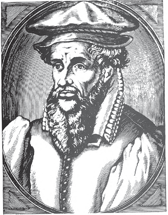
FIGURE 7.— Gerardus Mercator (1512-94). The inventor of the most famous map projection, which is the prototype for conformal mapping. — **FIGURE 7**.— Gerardus Mercator (1512-94). The inventor of the most famous map projection, which is the prototype for conformal mapping.

FEATURES AND USAGE #

The meridians of longitude of the Mercator projection are vertical parallel equally spaced lines, cut at right angles by horizontal straight parallels which are increasingly spaced toward each pole so that conformality exists (fig. 8). The spacing of parallels at a given latitude on the sphere is proportional to the secant of the latitude.

The major navigational feature of the projection is found in the fact that a sailing route between two points is shown as a straight line, if the direction or azimuth of the ship remains constant with respect to north. This kind of route is called a loxodrome or rhumb line and is usually longer than the great circle path (which is the shortest possible route on the sphere). It is the same length as a great circle only if it follows the Equator or a meridian. The projection has been standard since 1910 for nautical charts prepared by the former U.S. Coast and Geodetic Survey (now National Ocean Service) (Shalowitz, 1964, p. 302).

FIGURE 8.— The Mercator projection. The best-known projection. All angles are shown correctly, therefore, small shapes are essentially true, and it is called conformal. Since rhumb lines are shown straight on this projection, it is very useful in navigation. It is commonly used to show Equatorial regions of the Earth and other bodies.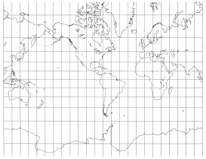 — **FIGURE 8**.— The Mercator projection. The best-known projection. All angles are shown correctly, therefore, small shapes are essentially true, and it is called conformal. Since rhumb lines are shown straight on this projection, it is very useful in navigation. It is commonly used to show Equatorial regions of the Earth and other bodies.

The great distortion of area on the Mercator projection of the Earth leads to mistaken concepts when it is the chief basis of world maps seen by students in school. The classic comparison of areas is between Greenland and South America. Greenland appears larger, although it is only one-eighth the size of South America. Furthermore, the North and South Poles cannot be shown, since they are at infinite distance from other parallels on the projection, giving a student an impression they are inaccessible (which of course they seemed to explorers long after the time of Mercator). The last 50 years have seen an increased emphasis on the use of other projections for world maps in published atlases.

Nevertheless, the Mercator projection is fundamental in the development of map projections, especially those which are conformal. It remains a standard navigational tool. It is also especially suitable for conformal maps of equatorial regions. The USGS has recently used it as an inset of the Hawaiian Islands on the 1:500,000-scale base map of Hawaii, for a Bathymetric Map of the Northeast Equatorial Pacific Ocean (although the projection is not stated) and for a Tectonic Map of the Indonesia region, the latter two both in 1978 and at a scale of 1:5,000,000.

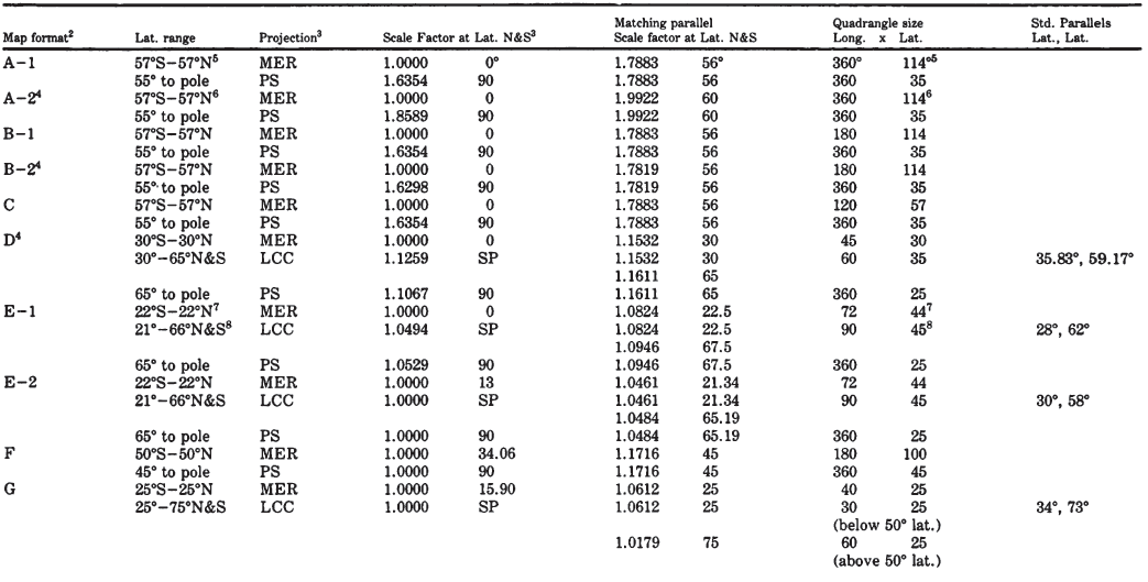
The first detailed map of an entire planet other than the Earth was issued in 1972 at a scale of 1:25,000,000 by the USGS Center of Astrogeology, Flagstaff, Arizona, following imaging of Mars by Mariner 9. Maps of Mars at other scales have followed. The mapping of the planet Mercury followed the flybys of Mariner 10 in 1974. Beginning in the late 1960’s, geology of the visible side of the Moon was mapped by the USGS in quadrangle fashion at a scale of 1:1,000,000. The four Galilean satellites of Jupiter and several satellites of Saturn were mapped following the Voyager missions of 1979-81. For all these bodies, the Mercator projection has been used to map equatorial portions, but coverage extended in some early cases to lats. 65" N. and S. (table 6).

TABLE 6.— Map projections used for extraterrestrial mapping — **TABLE 6**.— Map projections used for extraterrestrial mapping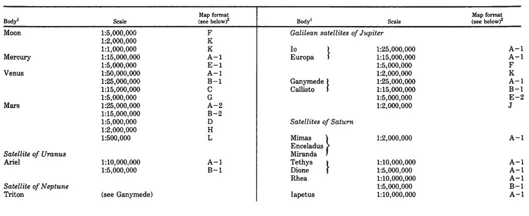

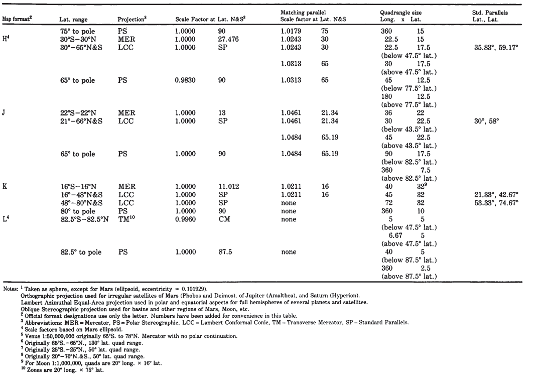
The cloudy atmosphere of Venus, circled by the Pioneer Venus Orbiter beginning in late 1978, is delaying more precise mapping of that planet, but the Mercator projection alone was used to show altitudes based on radar reflectivity over about 93 percent of the surface.

FORMULAS FOR THE SPHERE #

There is no suitable geometrical construction of the Mercator projection. For the sphere, the formulas for rectangular coordinates are as follows:

$$ x = R (\lambda - \lambda_0) \tag{ 7-1 } $$

$$ y = R \ln{\tan(\pi/4+\phi/2)} \tag{ 7-2 } $$

$$ y=(R/2)[ln((1+\sin\phi)/(1-\sin\phi))] \tag{ 7-2a } $$

where $R$ is the radius of the sphere at the scale of the map as drawn, and $\phi$ and $\lambda$ are given in radians. There are also several other forms in which equation (7-2) may he written, such as $y=R\,\mathrm{arcsinh}(\tan\phi) = R\, \mathrm{arctanh}(\sin\phi) = R \ln(\tan\phi+\sec\phi)$. The X axis lies along the Equator, x increasing easterly. The Y axis lies along the central meridian $\lambda_0$, y increasing northerly. If $(\lambda-\lambda_0)$ lies outside the range ±180°, 360° should be added or subtracted so it will fall inside the range. To use $\phi$ and $\lambda$ in degrees,

$$ x = \pi R (\lambda-\lambda_0)/180^\circ \tag{ 7-1a } $$

$$ y = R \ln\tan(45^\circ + \phi^\circ/2) \tag{ 7-2a } $$

$$ \eqalign{ h &= k = \sec\phi = 1/\cos\phi \cr \omega &= 0 } \tag{ 7-3 } $$

Normally, for conformal projections, the use of $h$ (the scale factor along a meridian) is omitted, and $k$ (the scale factor along a parallel) is used for the scale factor in any direction. The areal scale factor for conformal projections is $k^2$ or $\sec^2\phi$ for the Mercator in spherical form.

The inverse formulas for the sphere, to obtain $\phi$ and $\lambda$ from rectangular coordinates, are as follows:

$$ \phi = \pi/2 - 2\arctan(\mathrm{e}^{-y/R}) \tag{ 7-4 } $$

$$ \phi=\arctan[\sinh(y/R)] \tag{ 7-4a } $$

$$ \lambda = x/R + \lambda_0 \tag{ 7-5 } $$

Here $\mathrm{e} = 2.7182818\dots$, the base of natural logarithms, not eccentricity. These and subsequent formulas are given only in radians, as stated earlier, unless the degree symbol is used. Numerical examples (see numerical example) are given in degrees, showing conversion.

FORMULAS FOR THE ELLIPSOID #

For the ellipsoid, the corresponding equations for the Mercator are only a little more involved (see numerical example):

$$ x = a(\lambda-\lambda0) \tag{ 7-6 } $$

$$ y=a\ln{\left[\tan(\pi/4+\phi/2)\left(\frac{1-e\sin\phi}{1+e\sin\phi}\right)^{e/2}\right]} \tag{ 7-7 } $$

$$ y=(a/2)\ln\left[\left(\frac{1+\sin\phi}{1-\sin\phi}\right)\left(\frac{1-e\sin\phi}{1+e\sin\phi}\right)^e\right] \tag{ 7-7a } $$

where $a$ is the equatorial radius of the ellipsoid, and $e$ is its eccentricity. Comparing equation (3-7), it is seen that $y = a\psi$. From equations (4-22) and (4-23), it may be found that

$$ h = k = (1-e^2\sin^2\phi)^{1/2}/\cos\phi \tag{ 7-8 } $$

and of course $\omega=0$. The areal scale factor is $k^2$. The derivation of these equations is shown in Thomas (1952, p. 1, 2, 85-90).

The X and Y axes are oriented as they are for the spherical formulas, and $(\lambda-\lambda_0)$ should be similarly adjusted. Thomas also provides a series equivalent to equation (7-7), slightly modified here for consistency:

$$ \begin{align} y/a = &\ln {\tan(\pi/4+\phi/2)} - (e^2+e^4+e^6/8+\dots)\sin\phi \cr &+(e^4/12 + e^6/16+\dots)\sin{3\phi}-(e^6/80+\dots)\sin{5\phi}+\dots \end{align} \tag{ 7-7b } $$

The inverse formulas for the ellipsoid require rapidly converging iteration, if the closed forms of the equations for finding $\phi$ are used:

$$ \phi=\pi/2-2\arctan\{t[(1-e\sin\phi)/(1+e\sin\phi)]^{e/2}\} \tag{ 7-9 } $$

where:

$$ t=\mathrm{e}^{-y/a} \tag{ 7-10 } $$

$\mathrm{e}$ is the base of natural logarithms, 2.71828….,

at first trial

$$ \phi=\pi/2-2\arctan{t} \tag{ 7-11 } $$

Inserting the first trial $\phi$ in the right side of equation (7-9), $\phi$ on the left side is calculated. This becomes the new trial $\phi$, which is used on the right side. The process is repeated until the change in $\phi$ is less than a chosen convergence factor depending on the accuracy desired. This $\phi$ is then the final value. For $\lambda$,

$$ \lambda=x/a+\lambda_0 \tag{ 7-12 } $$

The scale factor is calculated from equation (7-8), using the calculated $\phi$. To avoid the iteration, the series (3-5) may be used with (7-13) in place of (7-9):

$$ \begin{align} \phi=&\chi+(e^2/2+5e^4/24+e^6/12+13e^8/360+\dots)\sin{2\chi}+ \cr &(7e^4/48+29e^6/240+811e^8/11520+\dots)\sin{4\chi}+ \cr &(7e^6/120+81e^8/1120+\dots)\sin{6\chi}+(4279e^8/161280+\dots)\sin{8\chi} \end{align} $$

where

$$ \chi=\pi/2-2\arctan t \tag{ 7-13 } $$

For improved computational efficiency using the series, see p. 19. Rectangular coordinates for each 5° of latitude are given in table 7, for both the sphere and the Clarke 1866 ellipsoid, assuming R and a are both 1.0.

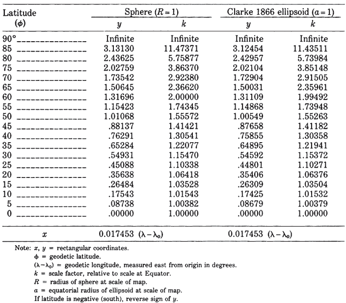
TABLE 7.— Mercator projection: Rectangular coordinates — **TABLE 7**.— Mercator projection: Rectangular coordinates

It should be noted that $k$ for the sphere applies only to the sphere. The spherical projection is not conformal with respect to the ellipsoidal Earth, although the variation is negligible for a map with an equatorial scale of 1:15,000,000 or smaller. It should be noted that any central meridian can be chosen as $\lambda_0$ for an existing Mercator map, if forward or inverse formulas are to be used for conversions.

MEASUREMENT OF RHUMB LINES #

Since a major feature of the Mercator projection is the straight portrayal of rhumb lines, formulas are given below to determine their true lengths and azimuths. If a straight line on the map connects two points with respective latitudes and longitudes $(\phi_1, \lambda_1)$ and $(\phi_2, \lambda_2)$, the respective rectangular coordinates $(x_1, y_1)$ and $(x_2, y_2)$ are calculated using equations (7-1) and (7-2) for the sphere or (7-6) and (7-7) for the ellipsoid, inserting the respective subscripts.

For the true (not magnetic) compass bearing or azimuth $Az$ clockwise from north along the rhumb line,

$$ Az = \arctan[(x_2-x_1)/(y_2-y_1)] \tag{ 7-14 } $$

Transposing and using forward and inverse equations for the Mercator, latitude or longitude along the rhumb line may be found for a given longitude or latitude, respectively, knowing the initial point and the azimuth. For example

$$ y_2 = y_1 + (x_2+x_1)/\tan{Az} \tag{ 7-15 } $$

in which $(x_1, y_1)$ are calculated for $(\phi_1, \lambda_1)$ from (7-6) and (7-7), $x_2$ is calculated from $\lambda_2$ (7-6), and $\phi_2$ is calculated from $y_2$ using (7-9) and (7-10).

For the true distance s along the rhumb line from $\phi_1$ to $\phi_2$,

$$ s = (M_2-M_1)/cos{Az} \tag{ 7-16 } $$

where $M_2$ and $M_1$, the distances from the Equator along the meridian, are found for $\phi_2$ and $\phi_1$, respectively, using equation (3-21) and the same subscripts on $M$ and $\phi$:

$$ \begin{align} M = a[&(1 - e^2/4 - 3e^4/64 - 5e^6/256 - \dots)\phi \\ -&(3e^2/8+3e^4/32+45e^6/1024+\dots)\sin{2\phi} \\ +&(15e^4/256+45e^6/1024+\dots)\sin{4\phi} - (35e^6/3072+\dots)\sin{6\phi}+\dots] \end{align} \tag{3-21} $$

but if $\phi_1 = \phi2$ equation (7-16) is indeterminate and

$$ s = a(\lambda_2-\lambda_1)\cos\phi/(1-e^2-\sin^2\phi)^{1/2} \tag{ 7-17 } $$

For the true distance $s$ from initial latitude $\phi_1$, to latitude $\phi_2$, equation (7-16) may be used with $M$ instead of $M_2$. To find $(\phi, \lambda)$ corresponding to a given distance $s$ from $(\phi_1, \lambda_1)$ along the rhumb line, (7-16) may be inverted to give:

$$ M=s\cos{Az}+M_1 \tag{ 7-18 } $$

$M$ may be converted to $\phi$ using (3-26),

$$ \begin{align} \phi = \mu &+ (3e_1/2-27e_1^3/32+\dots)\sin{2\mu}+(21e_1^2/16-55e_1^4/32+\dots)\sin{4\mu} \\ &+ (151e_1^3/96-\dots)\sin{6\mu}+(1097e_1^4/512-\dots)\sin{8\mu}+\dots \end{align} \tag{3-26} $$

where

$$ e_1 = [1-(1-e^2)^{1/2}]/[1+(1-e^2)^{1/2}] \tag{3-24} $$

and, in a rearrangement of (3-20) and (3-21),

$$ \mu=M/[a(1-e^2/4-3e^4/64-5e^6/256-\dots)] \tag{ 7-19 } $$

Then for longitude $\lambda$, rearranging (7-6), (7-7), and (7-14),

$$ \lambda=\lambda_1+\tan{Az}\ln\left[\tan(\pi/4+\phi/2)\left(\frac{1-e\sin\phi}{1+e\sin\phi}\right)^{e/2}\right] \tag{ 7-20 } $$

MERCATOR PROJECTION WITH ANOTHER STANDARD PARALLEL #

The above formulas are based on making the Equator of the Earth true to scale on the map. Thus, the Equator may be called the standard parallel. It is also possible to have, instead, another parallel (actually two) as standard, with true scale. For the Mercator, the map will look exactly the same; only the scale will be different. If latitude $\phi_1$, is made standard (the opposite latitude $-\phi_1$ is also standard), the above forward formulas are adapted by multiplying the right side of equations (7-1) through (7-3) for the sphere, including the alternate forms, by $\cos\phi_1$. For the ellipsoid, the right sides of equations (7-6), (7-7), (7-8), and (7-7a) are multiplied by $\cos\phi_1/(1-e^2\sin^2\phi_1)^{1/2}$. For inverse equations, divide $x$ and $y$ by the same values before use in equations (7-4) and (7-5) or (7-10) and (7-12). Such a projection is most commonly used for a navigational map of part of an ocean, such as the North Atlantic Ocean, but the USGS has used it for equatorial quadrangles of some extraterrestrial bodies as described in table 6.