8. TRANSVERSE MERCATOR PROJECTION #
SUMMARY #
- Cylindrical (transverse).
- Conformal.
- Central meridian, each meridian 90" from central meridian, and Equator are straight lines.
- Other meridians and parallels are complex curves.
- Scale is true along central meridian, or along two straight lines equidistant from and parallel to central meridian. (These lines are only approximately straight for the ellipsoid.)
- Scale becomes infinite on sphere 90° from central meridian.
- Used extensively for quadrangle maps at scales from 1:24,000 to 1:250,000.
- Presented by Lambert in 1772.
HISTORY #
Since the regular Mercator projection has little error close to the Equator (the scale 10° away is only 1.5 percent larger than the scale at the Equator), it has been found very useful in the transverse form, with the equator of the projection rotated 90° to coincide with the desired central meridian. This is equivalent to wrapping the cylinder around a sphere or ellipsoid representing the Earth so that it touches the central meridian throughout its length, instead of following the Equator of the Earth. The central meridian can then be made true to scale, no matter how far north and south the map extends, and regions near it are mapped with low distortion. Like the regular Mercator, the map is conformal.
The Transverse Mercator projection in its spherical form was invented by the prolific Alsatian mathematician and cartographer Johann Heinrich Lambert (1728-77) (fig. 9). It was the third of seven new projections which he described in 1772 in his classic Beitrage (Lambert, 1772). At the same time, he also described what are now called the Cylindrical Equal-Area, the Lambert Conformal Conic, and the Lambert Azimuthal Equal-Area, each of which will be discussed subsequently; others are omitted here. He described the Transverse Mercator as a conformal adaptation of the Sinusoidal projection, then commonly in use (Lambert, 1772, p. 57-58). Lambert’s derivation was followed with a table of coordinates and a map of the Americas drawn according to the projection.
Little use has been made of the Transverse Mercator for single maps of continental areas. While Lambert only indirectly discussed its ellipsoidal form, mathematician Carl Friedrich Gauss (1777-1855) analyzed it further in 1822, and L. Krüger published studies in 1912 and 1919 providing formulas suitable for calculation relative to the ellipsoid. It is, therefore, sometimes called the Gauss Conformal or the Gauss-Krüger projection in Europe, but Transverse Mercator, a term first applied by the French map projection compiler Germain, is the name normally used in the United States (Thomas, 1952, p. 91-92; Germain, 1865?, p. 347).
Until recently, the Transverse Mercator projection was not precisely applied to the ellipsoid for the entire Earth. Ellipsoidal formulas were limited to series for relatively narrow bands. In 1945, E. H. Thompson (and in 1962, L. P. Lee) presented exact or closed formulas permitting calculation of coordinates for the full ellipsoid, although elliptic functions, and therefore lengthy series, numerical integrations, and (or) iterations, are involved (Lee, 1976, p. 92-101; Snyder, 1979a, p. 73; Dozier, 1980).
The formulas for the complete ellipsoid are interesting academically, but they are practical only within a band between 4° of longitude and some 10° to 15° of arc distance on either side of the central meridian, because of the much more significant scale errors fundamental to any projection covering a larger area. FIGURE 9.— Johann Heinrich Lambert (1728-77). Inventor of the Transverse Mercator, the Conformal Conic, the Azimuthal Equal-Area, and other important projections, as well as outstanding developments in mathematics, astronomy, and physics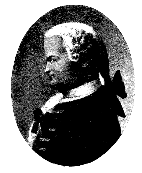
FEATURES #
The meridians and parallels of the Transverse Mercator (fig. 10) are no longer the straight lines they are on the regular Mercator, except for the Earth’s Equator, the central meridian, and each meridian 90° away from the central meridian. Other meridians and parallels are complex curves.
The spherical form is conformal, as is the parent projection, and scale error is only a function of the distance from the central meridian, just as it is only a function of the distance from the Equator on the regular Mercator. The ellipsoidal form is also exactly conformal, but its scale error is slightly affected by factors other than the distance alone from the central meridian (Lee, 1976, p. 98). FIGURE 10.— The Transverse Mercator projection. While the regular Mercator has constant scale along the Equator, the Transverse Mercator has constant scale along any chosen central meridian. This projection is conformal and is often used to show regions with greater north-south extent.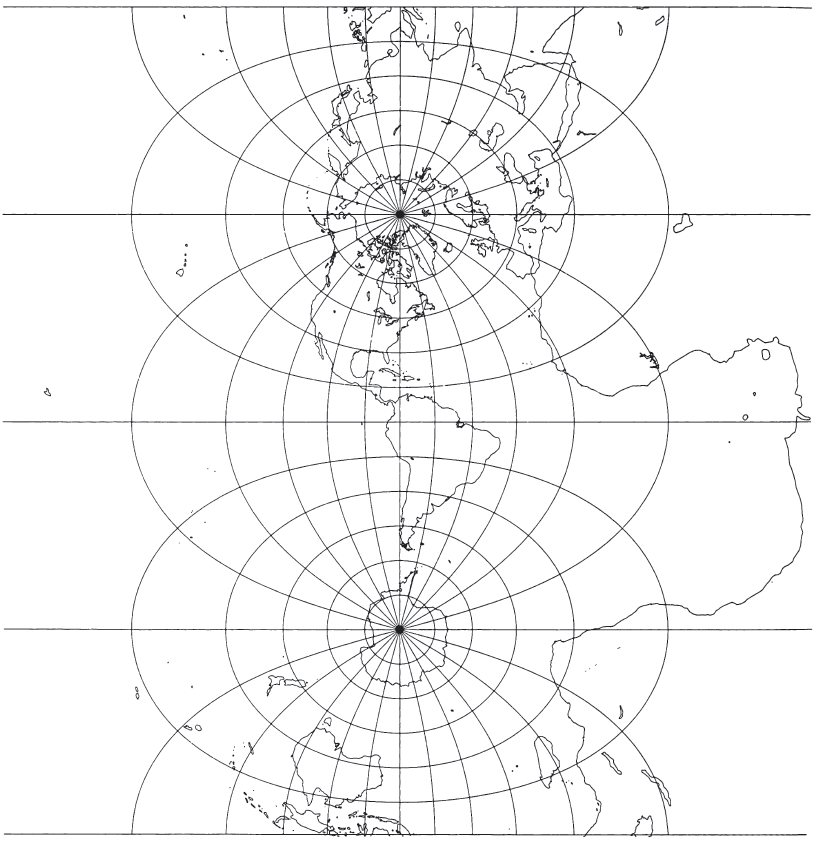
With the scale along the central meridian remaining constant, the Transverse Mercator is an excellent projection for lands extending predominantly north and south.
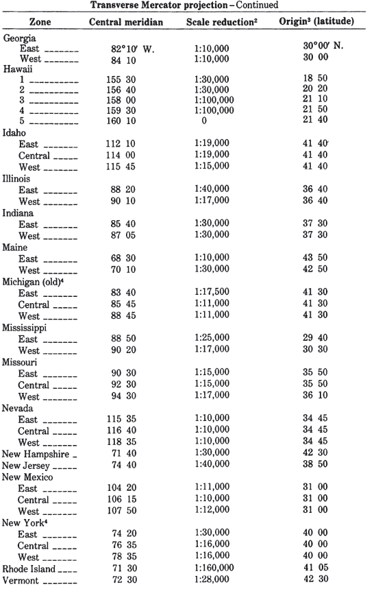
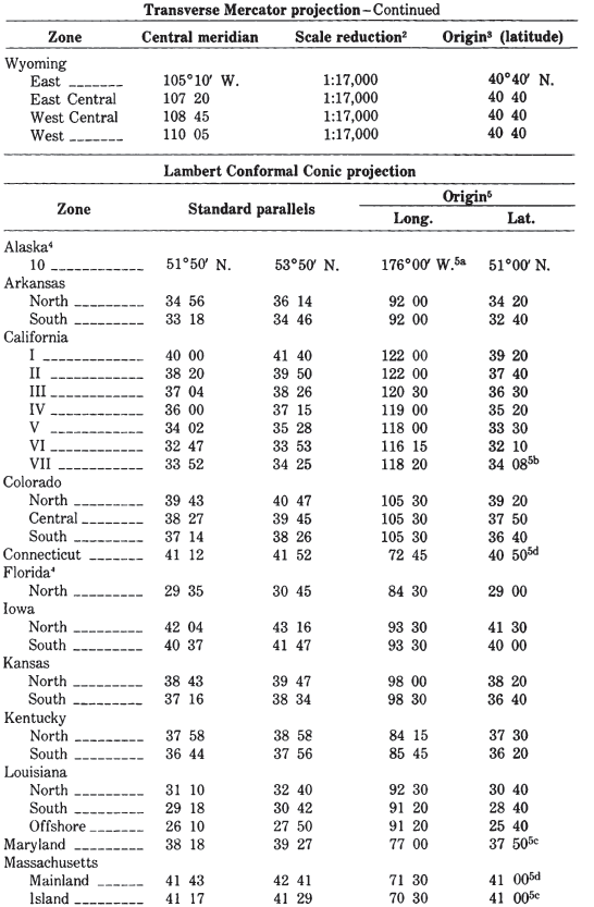
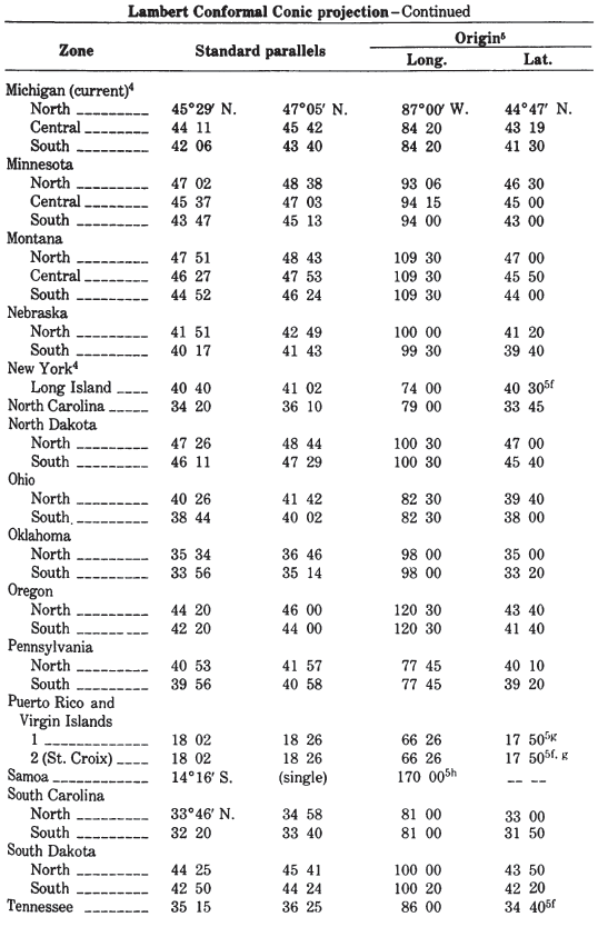
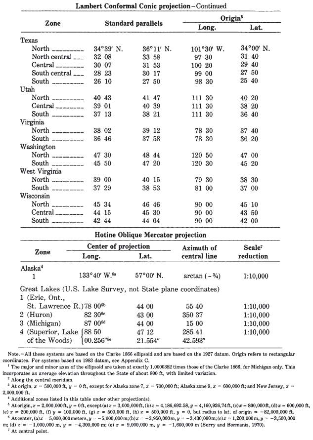
TABLE 8.— U.S. State plane coordinate systems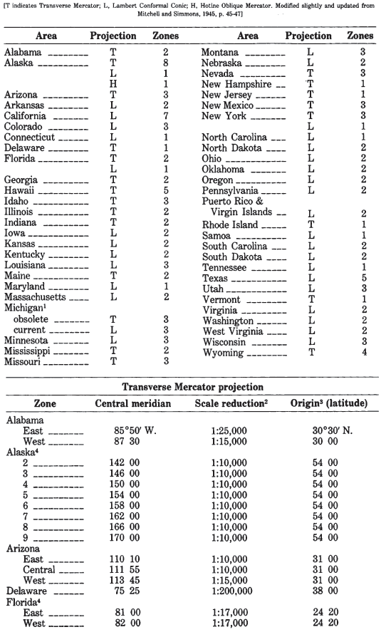
USAGE #
The Transverse Mercator projection (spherical or ellipsoidal) was not described by Close and Clarke in their generally detailed article in the 1911 Encyclopaedia Britannica because it was “seldom used” (Close and Clarke, 1911, p. 663). Deetz and Adams (1934) favorably referred to it several times, but as a slightly used projection.
The spherical form of the Transverse Mercator has been used by the USGS only recently. In 1979, this projection was chosen for a base map of North America at a scale of 1:5,000,000 to replace the Bipolar Oblique Conic Conformal projection previously used for tectonic and other geologic maps. The scale factor along the central meridian, long. 100° W., is reduced to 0.926. The radius of the Earth is taken at 6,371,204 m, with approximately the same surface area as the International ellipsoid, placing the two straight lines of true design scale 2,343 km on each side of the central meridian.
While its use in the spherical form is limited, the ellipsoidal form of the Transverse Mercator is probably used more than any other one projection for geodetic mapping.
In the United States, it is the projection used in the State Plane Coordinate System (SPCS) for States with predominant north-south extent. (The Lambert Conformal Conic is used for the others, except for the panhandle of Alaska, which is prepared on the Oblique Mercator. Alaska, Florida, and New York use both the Transverse Mercator and the Lambert Conformal Conic for different zones.) Except for narrow States, such as Delaware, New Hampshire, and New Jersey, all States using the Transverse Mercator are divided into two to eight zones, each with its own central meridian, along which the scale is slightly reduced to balance the scale throughout the map. Each zone is designed to maintain scale distortion within 1 part in 10,000. Several States beginning in 1935 also passed legislation establishing the SPCS as a permissible system for recording boundary descriptions or point locations. Several zone changes have occurred for use with the new 1983 datum. They are listed in Appendix C.
In addition to latitude and longitude as the basic frame of reference, the corresponding rectangular grid coordinates in feet are used to designate locations (Mitchell and Simmons, 1945). The parameters for each State are given in table 8. All are based on the Clarke 1866 ellipsoid. It is important to note that, for the metric conversion to feet using this coordinate system, 1 m equals exactly 39.37in., not the current standard accepted by the National Bureau of Standards in 1959, in which 1 in. equals exactly 2.54 cm. Surveyors continue to follow the former conversion for consistency. The difference is only two parts in a million, but it is enough to cause confusion, if it is not accounted for.
Beginning with the late 1950’s, the Transverse Mercator projection was used by the USGS for nearly all new quadrangles (maps normally bounded by meridians and parallels) covering those States using the TM Plane Coordinates, but the central meridian and scale factor are those of the SPCS zone. Thus, all quadrangles for a given zone may be mosaicked exactly. Beginning in 1977, many USGS maps have been produced on the Universal Transverse Mercator projection (see below). Prior to the late 1950’s, the Polyconic projection was used. The change in projection was facilitated by the use of high-precision rectangular-coordinate plotting machines. Some maps produced on the Transverse Mercator projection system during this transition period are identified as being prepared according to the Polyconic projection. Since most quadrangles cover only 7½ minutes (at a scale of 1:24,000) or 15 minutes (at 1:62,500) of latitude and longitude, the difference between the Polyconic and the Transverse Mercator for such a small area is much more significant due to the change of central meridian than due to the change of projection. The difference is still slight and is detailed later under the discussion of the Polyconic projection. The Transverse Mercator is used in many other countries for official topographic mapping as well. The Ordnance Survey of Great Britain began switching from a Transverse Equidistant Cylindrical (the Cassini-Soldner) to the Transverse Mercator about 1920.
The use of the Transverse Mercator for quadrangle maps has been recently extended by the USGS to include the planet Mars. Although other projections are used at smaller scales, quadrangles at scales of 1:1,000,000 and 1:250,000, and covering areas from 200 to 800 km on a side, were drawn to the ellipsoidal Transverse Mercator between lats. 65°N. and S. The scale factor along the central meridian was made 1.0. For the current series, see table 6.
In addition to its own series of larger-scale quadrangle maps, the Army Map Service used the Transverse Mercator for two other major mapping operations:
(1) a series of 1:250,000-scale quadrangle maps covering the entire country, and
(2) as the geometric basis for the Universal Transverse Mercator (UTM) grid.
The entire area of the United States has been mapped since the 1940’s in sections 2° of longitude (between even-numbered meridians, but in 3° sections in Alaska) by 1° of latitude (between each full degree) at a scale of 1:250,000, with the UTM grid superimposed and with some variations in map boundaries at coastlines. These maps were drawn with reference to their own central meridians, not the central meridians of the UTM zones (see below), although the 0.9996 central scale factor was employed. The central meridian of about one-third of the maps coincides with the central meridian of the zone, but it does not for about two-thirds, the “wing” sheets, which therefore do not perfectly match the center sheets. The USGS has assumed publication and revision of this series and is casting new maps using the correct central meridians.
Transverse Mercator quadrangle maps fit continuously in a north-south direction, provided they are prepared at the same scale, with the same central meridian, and for the same ellipsoid. They do not fit exactly from east to west, if they have their own central meridians; although quadrangles and other maps properly constructed at the same scale, using the SPCS or UTM projection, fit in all directions within the same zone.
UNIVERSAL TRANSVERSE MERCATOR PROJECTION #
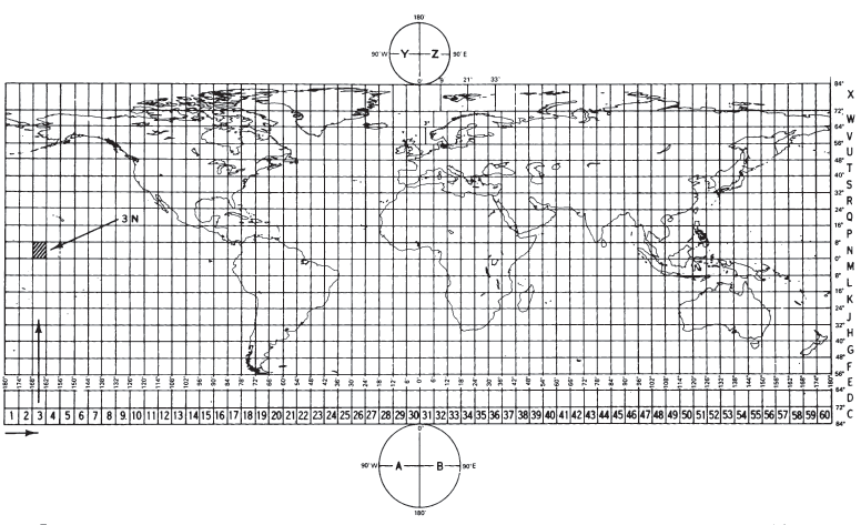
The Universal Transverse Mercator (UTM) projection and grid were adopted by the U.S. Army in 1947 for designating rectangular coordinates on large-scale military maps of the entire world. The UTM is the ellipsoidal Transverse Mercator to which specific parameters, such as central meridians, have been applied. The Earth, between lats. 84° N. and 80° S., is divided into 60 zones each generally 6° wide in longitude. Bounding meridians are evenly divisible by 6°, and zones are numbered from 1 to 60 proceeding east from the 180th meridian from Greenwich with minor exceptions. There are letter designations from south to north (see fig. 11). Thus, Washington, D.C., is in grid zone 18S, a designation covering a quadrangle from long. 72° to 78° W. and from lat. 32° to 40° N. Each of these quadrangles is further subdivided into grid squares 100,000 meters on a side with double-letter designations, including partial squares at the grid boundaries. From lat. 84° N. and 80° S. to the respective poles, the Universal Polar Stereographic (UPS) projection is used instead.
As with the SPCS, each geographic location in the UTM projection is given $x$ and $y$ coordinates, but in meters, not feet, according to the Transverse Mercator projection, using the meridian halfway between the two bounding meridians as the central meridian, and reducing its scale to 0.9996 of true scale (a 1:2,500 reduction). The reduction was chosen to minimize scale variation in a given zone; the variation reaches 1 part in 1,000 from true scale at the Equator. The USGS, for civilian mapping, uses only the zone number and the $x$ and $y$ coordinates, which are sufficient to define a point, if the ellipsoid and the hemisphere (north or south) are known; the 100,000-m square identification is not essential. The lines of true scale are approximately parallel to and approximately 180 km east and west of the central meridian. Between them, the scale is too small; beyond them, it is too great. In the Northern Hemisphere, the Equator at the central meridian is considered the origin, with an $x$ coordinate of 500,000 m and a $y$ of 0. For the Southern Hemisphere, the same point is the origin, but, while $x$ remains 500,000 m, $y$ is 10,000,000 m. In each case, numbers increase toward the east and north. Negative coordinates are thus avoided (Army, 1973, p. 7, endmap). A page of coordinates for the UTM projection is shown in table 9. TABLE 9.— Universal Transverse Mercator grid coordinates FIGURE 11.— Universal Transverse Mercator (UTM) grid zone designations for the world shown on a horizontally expanded Equidistant Cylindrical projection index map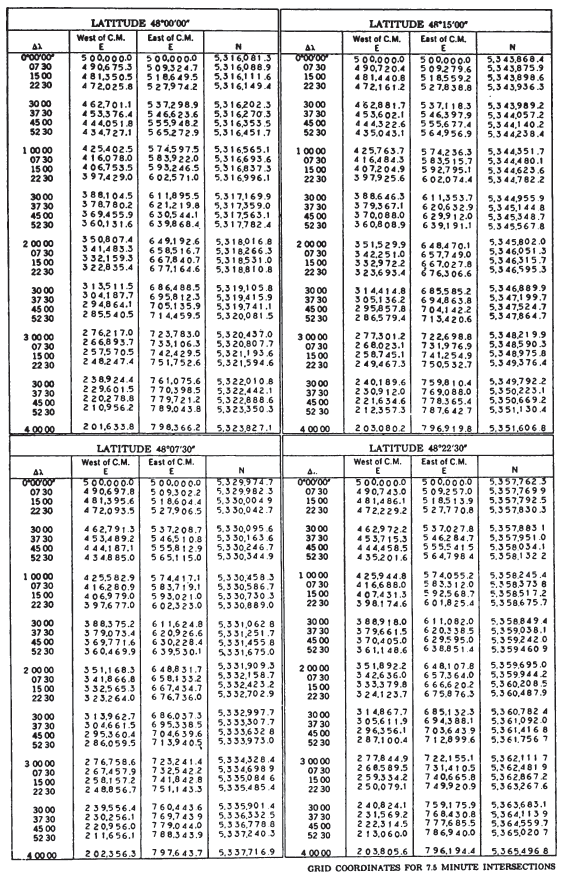
The ellipsoidal Earth is used throughout the UTM projection system, but the reference ellipsoid changes with the particular region of the Earth. For all land under United States jurisdiction, the Clarke 1866 ellipsoid is used for the map projection. For the UTM grid superimposed on the map of Hawaii, however, the International ellipsoid is used. The Geological Survey uses the UTM graticule and grid for its 1:250,000- and larger-scale maps of Alaska, and applies the UTM grid lines or tick marks to its quadrangles and State base maps for the other States, although they are generally drawn with different projections or parameters.
FORMULAS FOR THE SPHERE #
A partially geometric construction of the Transverse Mercator for the sphere involves constructing a regular Mercator projection and using a transforming map to convert meridians and parallels on one sphere to equivalent meridians and parallels on a sphere rotated to place the equator of one along the chosen central meridian of the other. Such a transforming map may be the equatorial aspect of the Stereographic or other azimuthal projection, drawn twice to the same scale on transparencies. The transparencies may then be superimposed at 90° angles and the points compared.
In an age of computers, it is much more satisfactory to use mathematical formulas. The rectangular coordinates for the Transverse Mercator applied to the sphere (Thomas, 1952, p. 6):
The inverse formulas for$(\phi,\lambda)$ in terms of $(x,y)$:
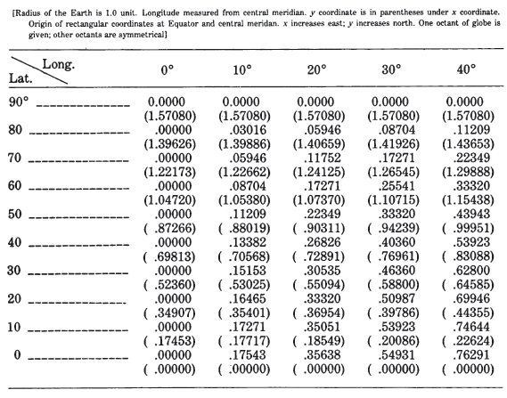
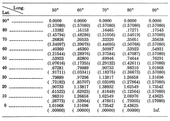
TABLE 10.— Transverse Mercator projection: Rectangular coordinates for the sphere
FORMULAS FOR THE ELLIPSOID #
For the ellipsoidal form, the most practical form of the equations is a set of series approximations which converge rapidly to the correct centimeter or less at full scale in a zone extending 3° to 4° of longitude from the central meridian. Beyond this, the forward series as given here is accurate to about a centimeter at 7° longitude, but the inverse series does not have sufficient terms for this accuracy. The forward series may be used with meter accuracy to 10° of longitude. (Many additional terms for use to 24° of longitude may be found in Army (1962).) Coordinate axes are the same as they are for the spherical formulas above. The formulas below are only slightly modified from those presented in standard references to provide mm accuracy at full scale (Army, 1973, p. 5-7; Thomas, 1952, p. 2-3). (See numerical examples)
$M_0 = M$ calculated for $\phi_0$ the latitude crossing the central meridian $\lambda_0$ at the origin of the $x, y$ coordinates. Note: If $\phi=\pm\pi/2$, all equations should be omitted except (3-21), from which $M$ and $M_0$ are calculated. Then $x=0, y=k_0(M-M_0), k=k_0$.
Equation (8-11) for $k$ may also be written as a function of $x$ and $\phi$:
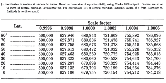
TABLE 11.— Universal Transverse Mercator projection: Location of points with given scale factor
To obtain UTM or SPCS coordinates, the appropriate “false easting” is added to $x$ and “false northing” added to $y$ after calculation using (8-9) and (8-10).
For the inverse formulas (Army, 1973, p. 6, 7, 46; Thomas, 1952, p. 2-3):
It may be found from equation (3-26):
For improved computational efficiency using series (3-21) and (3-26), see p. 19. From $\phi_1$, other terms below are calculated for use in equations (8-17) and (8-18). (If $\phi_1 = \pm\pi/2$, (8-12), (8-21) through (8-25), (8-17) and (8-18) are omitted, but $\phi=\pm90°$ taking the sign of $y$, while $\lambda$ is indeterminate, and may be called $\lambda_0$. Also, $k = k_0$.)
“MODIFIED TRANSVERSE MERCATOR” PROJECTION #
In 1972, the USGS devised a projection specifically for the revision of a 1954 map of Alaska which, like its predecessors, was based on the Polyconic projection. The projection was drawn to a scale of 1:2,000,000 and published at 1:2,500,000 (map “E”) and 1:1,584,000 (map “B”). Graphically prepared by adapting coordinates for the Universal Transverse Mercator projection, it is identified as the “Modified Transverse Mercator” projection. It resembles the Transverse Mercator in a very limited manner and cannot be considered a cylindrical projection. It approximates an Equidistant Conic projection for the ellipsoid in actual construction. Because of the projection name, it is listed here. The projection was also used in 1974 for a base map of the Aleutian-Bering Sea Region published at the 1:2,500,000 scale.
The basis for the name is clear from an unpublished 1972 description of the projection, in which it is also stressed that the “latitudinal lines are parallel” and the “longitudinal lines are straight.” The computations
were taken from the AMS Technical Manual #21 (Universal Transverse Mercator) based on the Clarke 1866 Spheroid.*** The projection was started from a N-S central construction line of the 153° longitude which is also the centerline of Zone 5 from the UTM tables. Along this line each even degree latitude was plotted from book values. At the plotted point for the 64° latitude, a perpendicular to the construction line (153°) was plotted. From the center construction line for each degree east and west for 4° (the limits of book value of Zone #5) the curvature of latitude was plotted. From this 64° latitude, each 2° latitude north to 70° and south to 54° was constructed parallel to the 64° latitude line. Each degree of longitude was plotted on the 58° and 68° latitude line. Through corresponding degrees of longitude along these two lines of latitude a straight line (line of longitude) was constructed and projected to the limits of the map. This gave a small projection 8° in width and approximately 18° in length. This projection was repeated east and west until a projection of some 72° in width was attained.
For transferring data to and from the Alaska maps, it was necessary to determine projection formulas for computer programming. Since it appeared to be unnecessarily complicated to derive formulas based on the above construction, it was decided to test empirical formulas with actual coordinates. After careful measurements of coordinates for graticule intersections were made in 1979 on the stable-base map, it was determined that the parallels very closely approximate concentric circular arcs, spaced in proportion to their true distances on the ellipsoid, while the meridians are nearly equidistant straight lines radiating from the center of the circular arcs. Two parallels have a scale equal to that along the meridians. The Equidistant Conic projection for the ellipsoid with two standard parallels was then applied to these coordinates as the closest approximation among projections with available formulas. After various trial values for scale and standard parallels were tested, the empirical formulas below (equations (8-26) through (8-32)) were obtained. These agree with measured values within 0.005 inch at mapping scale for 44 out of 58 measurements made on the map and within 0.01 inch for 54 of them.
FORMULAS FOR THE “MODIFIED TRANSVERSE MERCATOR” PROJECTION #
The “Modified Transverse Mercator” projection was found to be most closely equivalent to an Equidistant Conic projection for the Clarke 1866 ellipsoid, with the scale along the meridians reduced to 0.9992 of true scale and the standard parallels at lat. 66.09° and 53.50° N. (also at 0.9992 scale factor). For the Alaska Map “E” at 1:2,500,000, using long. 150° W. as the central meridian and lat. 58° N. as the latitude of the origin on the central meridian, the general formulas (Snyder, 1978a, p. 378) reduce with the above parameters to the following, giving x and y in meters at the map scale. The Y axis lies along the central meridian, y increasing northerly, and the X axis is perpendicular at the origin, x increasing easterly.
The equation for $\phi$, (8-31), involves iteration by successive substitution. If an initial $\phi$ of 60° is inserted into the right side, $\phi$ on the left may be calculated and substituted into the right in place of the previous trial $\phi$. Recalculations continue until the change in $\phi$ is less than a preset convergence. If $\lambda$ as calculated is less than -180°, it should be added to 360° and labeled East Longitude.
Formulas to adjust $x$ and $y$ for the map inset of the Aleutian Islands are omitted here, but the coordinates above are rotated counterclockwise 29.79° and transposed to + 0.798982 m for x and + 0.347600 m for y.