9. OBLIQUE MERCATOR PROJECTION #
SUMMARY #
- Cylindrical (oblique).
- Conformal.
- Two meridians 180° apart are straight lines.
- Other meridians and parallels are complex curves.
- Scale on the spherical form is true along chosen central line, a great circle at an oblique angle, or along two straight lines parallel to central line. The scale on the ellipsoidal form is similar, but varies slightly from this pattern.
- Scale becomes infinite 90° from the central line.
- Used for grids on maps of the Alaska panhandle, for mapping in Switzerland, Madagascar, and Borneo and for atlas maps of areas with greater extent in an oblique direction.
- Developed 1900-50 by Rosenmund, Laborde, Hotine, and others.
HISTORY #
There are several geographical regions such as the Alaska panhandle centered along lines which are neither meridians nor parallels, but which may be taken as great circle routes passing through the region. If conformality is desired in such cases, the Oblique Mercator is a projection which should be considered.
The historical origin of the Oblique Mercator projection does not appear to be sharply defined, although it is a logical generalization of the regular and Transverse Mercator projections. Apparently, Rosenmund (1903) made the earliest published reference, when he devised an ellipsoidal form which is used for topographic mapping of Switzerland. The projection was not mentioned in the detailed article on “Map Projections” in the 1911 Encyclopaedia Britannica (Close and Clarke, 1911) or in Hinks’ brief text (1912). Laborde applied the Oblique Mercator to the ellipsoid for the topographic mapping of Madagascar in 1928 (Young, 1930; Laborde, 1928). H. J. Andrews (1935, 1938) proposed the spherical forms for maps of the United States and Eurasia. Hinks presented seven world maps on the Oblique Mercator, with poles located in several different positions, and a consequent variety in the regions shown more satisfactorily (Hinks, 1940, 1941).
A study of conformal projections of the ellipsoid by British geodesist Martin Hotine (1898-1968), published in 1946-47, is the basis of the U.S. use of the ellipsoidal Oblique Mercator, which Hotine called the “rectified skew orthomorphic” (Hotine, 1947, p. 66-67). The Hotine approach has limitations, as discussed below, but it provides closed formulas which have been adapted for U. S. mapping of suitable zones. One of its limitations is overcome by a recent series form of the ellipsoidal Oblique Mercator (Snyder, 1979a, p. 74), but other limitations result instead. This later form resulted from development of formulas for the continuous mapping of satellite images, using the Space Oblique Mercator projection (to be discussed later).
While Hotine projected the ellipsoid conformally onto an “aposphere” of constant total curvature and thence to a plane, J. H. Cole (1943, p. 16-30) projected the ellipsoid onto a “conformal sphere,” using conformal latitudes (described earlier) to make the sphere conformal with respect to the ellipsoid, then plotted the spherical Oblique Mercator from this intermediate sphere. Rosenmund’s system for Switzerland is a more complex double projection through a conformal sphere
(Rosenmund, 1903; Bolliger, 1967). Laborde combined the conformal sphere with a complex-algebra transformation of the Oblique Mercator (Reignier, 1957, p. 130). FIGURE 12.— Oblique Mercator projection with the center of projection at lat. 45° N. on the central meridian. A straight line through the point and, in this example, perpendicular to the central meridian is true to scale. The projection is conformal and has been used for regions lying along a line oblique to meridians.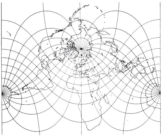
FEATURES #
The Oblique Mercator for the sphere is equivalent to a regular Mercator projection which has been altered by wrapping a cylinder around the sphere so that it touches the surface along the great circle path chosen for the central line, instead of along the Earth’s Equator. A set of transformed meridians and parallels relative to the great circle may be plotted bearing the same relationship to the rectangular coordinates for the Oblique Mercator projection, as the geographic meridians and parallels bear to the regular Mercator. It is, therefore, possible to convert the geographic meridians and parallels to the transformed values and then to use the regular Mercator equations, substituting the transformed values in place of the geographic values. This is the procedure for the sphere, although combined formulas are given below, but it becomes much more complicated for the ellipsoid. The advent of present-day computers and programmable pocket calculators make these calculations feasible for sphere or ellipsoid.
The resulting Oblique Mercator map of the world (fig. 12) thus resembles the regular Mercator with the landmasses rotated so that the poles and Equator are no longer in their usual positions. Instead, two points 90° away from the chosen great circle path through the center of the map are at infinite distance off the map. Normally, the Oblique Mercator is used only to show the region near the central line and for a relatively short portion of the central line. Under these conditions, it looks similar to maps of the same area using other projections, except that careful scale measurements will show differences.
It should be remembered that the regular Mercator is in fact a limiting form of the Oblique Mercator with the Equator as the central line, while the Transverse Mercator is another limiting form of the Oblique with a meridian as the central line. As with these limiting forms, the scale along the central line of the Oblique Mercator may be reduced to balance the scale throughout the map.
USAGE #
The Oblique Mercator projection is used in the spherical form for a few atlas maps. For example, the National Geographic Society uses it for atlas and sheet maps of Hawaii, the West Indies, and New Zealand. The spherical form is being used by the USGS for maps of North and South America and Australasia in a new set of 1:10,000,000-scale maps of Hydrocarbon Provinces. For North America, the central scale factor is 0.968, and the transformed pole is at lat. 10°N, long. 10°E. For South America, these numbers are 0.974, 10°N., and 30°E., respectively; for Australasia, 0.978, 55°N, and 160°W. These parameters were chosen after a least-squares analysis of over 100 points on each continent to determine optimum parameters for a common conformal projection.
In the ellipsoidal form it was used, as mentioned above, by Rosenmund for Switzerland and Laborde for Madagascar. Hotine used it for Malaya and Borneo and Cole for Italy. It is used in the Hotine form by the USGS for grid marks on zone 1 (the panhandle) of Alaska, using the State Plane Coordinate System as adapted to this projection by Erwin Schmid of the former Coast and Geodetic Survey. The Hotine form was also adopted by the U.S. Lake Survey for mapping of the five Great Lakes, the St. Lawrence River, and the U.S.-Canada Border Lakes west to the Lake of the Woods (Berry and Bormanis, 1970). Four zones are involved; see table 8 for parameters of these and the Alaska zones. TABLE 12.— Hotine Oblique Mercator projection parameters used for Landsat 1, 2, and 3 imagery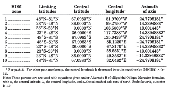
More recently, the Hotine form was adapted by John B. Rowland (USGS) for mapping Landsat 1, 2, and 3 satellite imagery in two sets of five discontinuous zones from north to south (table 12). The central line of the latter is only a close approximation to the satellite groundtrack, which does not follow a great circle route on the Earth; instead, it follows a path of constantly changing curvature. Until the mathematical implementation of the Space Oblique Mercator (SOM) projection, the Hotine Oblique Mercator (HOM) was probably the most suitable projection available for mapping Landsat type data. In addition to Landsat, the HOM projection has been used to cast Heat Capacity Mapping Mission (HCMM) imagery since 1978. NOAA (National Oceanic and Atmospheric Administration) has also cast some weather satellite imagery on the HOM to make it compatible with Landsat in the polar regions which are beyond Landsat coverage (above lat. 82°).
The parameters for a given map according to the Oblique Mercator projection may be selected in various ways. If the projection is to be used for the map of a smaller region, two points located near the limits of the region may be selected to lie upon the central line, and various constants may be calculated from the latitude and longitude of each of the two points. A second approach is to choose a central point for the map and an azimuth for the central line, which is made to pass through the central point. A third approach, more applicable to the map of a large portion of the Earth’s surface, treated as spherical, is to choose a location on the original sphere of the pole for a transformed sphere with the central line as the equator. Formulas are given for each of these approaches, for sphere and ellipsoid.
FORMULAS FOR THE SPHERE #
Starting with the forward equations, for rectangular coordinates in terms of latitude and longitude (see numerical examples):
Given two points to lie upon the central line, with latitudes and longitudes $(\phi_1,\lambda_1)$ and $(\phi_2,\lambda_2)$ and longitude increasing easterly and relative to Greenwich. The pole of the oblique transformation at $(\phi_p,\lambda_p)$ may be calculated as follows:
$$ \begin{align} \lambda_p = &\arctan[(\cos\phi_1\sin\phi_2\cos\lambda_1 - \sin\phi_1\cos\phi_2\cos\lambda_2)/ \\ &(\sin\phi_1\cos\phi_2\sin\lambda_2 - \cos\phi_1\sin\phi_2\sin\lambda_1)] \end{align} \tag{ 9-1 } $$$$ \phi_p = \arctan[-\cos(\lambda_p-\lambda_1)/\tan\phi_1] \tag{ 9-2 } $$The Fortran ATAN2 function or its equivalent should be used with equation (9-1), but not with (9-2). The other pole is located at $(-\phi_p,\lambda_p\pm\pi)$. Using the positive (northern) value of $\phi_p$, the following formulas give the rectangular coordinates for point $(\phi,\lambda)$, with $k_0$, the scale factor along the central line:$$ x = Rk_0\arctan\{[\tan\phi\cos\phi_p+\sin\phi_p\sin(\lambda-\lambda_0)]/\cos(\lambda-\lambda_0)\} \tag{ 9-3 } $$$$ y = (R/2)k_0\ln[(1+A)/(1-A)] \tag{ 9-4 } $$or$$ y=Rk_0\mathrm{arctanh}A \tag{ 9-4a } $$$$ k=k_0/(1-A^2)^{1/2} \tag{ 9-5 } $$where$$ A=\sin\phi_p\sin\phi - \cos\phi_p\cos\phi\sin(\lambda-\lambda_0) \tag{ 9-6 } $$With these formulas, the origin of rectangular coordinates lies at$$ \begin{align} \phi_0 &= 0 \\ \lambda_0 &=\lambda_p + \pi/2 \end{align} \tag{ 9-6a } $$and the X axis lies along the central line, $x$ increasing easterly. The transformed poles are $y$ equals infinity.Given a central point $(\phi_c,\lambda_c)$ with longitude increasing easterly and relative to Greenwich, and azimuth $\beta$ east of north of the central line through $(\phi_c,\lambda_c)$, the pole of the oblique transformation at $(\phi_p,\lambda_p)$ may be calculated as follows:
$$ \phi_p = \arcsin(\cos\phi_c\sin\beta) \tag{ 9-7 } $$$$ \lambda_p = \arctan[-\cos\beta/(-\sin\phi_c\sin\beta)]+ \lambda_c \tag{ 9-8 } $$These values of $\phi_p$ and $\lambda_p$, may then be used in equations (9-3) through (9-6) as before.For an extensive map, $\phi_p$ and $\lambda_p$ may be arbitrarily chosen by eye to give the pole for a central line passing through a desired portion of the globe. These values may then be directly used in equations (9-3) through (9-6) without intermediate calculation.
For the inverse formulas, equations (9-1) and (9-2) or (9-7) and (9-8) must first be used to establish the pole of the oblique transformation, if it is not known already. Then,
FORMULAS FOR THE ELLIPSOID #
These are the formulas provided by Hotine, slightly altered to use a positive eastern longitude (he used positive western longitude), to simplify calculations of hyperbolic functions, and to use symbols consistent with those of this bulletin. The central line is a geodesic, or the shortest route on an ellipsoid, corresponding to a great circle route on the sphere.
It is customary to provide rectangular coordinates for the Hotine in terms either of $(u, v)$ or $(x, y)$. The $(u, v)$ coordinates are similar in concept to the $(x, y)$ calculated for the foregoing spherical formulas, with $u$ corresponding to $x$ for the spherical formulas, increasing easterly from the origin along the central line, but $v$ corresponds to $-y$ for the spherical formulas, so that $v$ increases southerly in a direction perpendicular to the central line. For the Hotine, $x$ and $y$ are calculated from $(u, v)$ as “rectified” coordinates with the Y axis following the meridian passing through the center point, and increasing northerly as usual, while the X axis lies east and west through the same point. The X and Y axes thus lie in directions like those of the Transverse Mercator, but the scale-factor relationships remain those of the Oblique Mercator.
The normal origin for $(u, v)$ coordinates in the Hotine Oblique Mercator is approximately at the intersection of the central line wilh the Earth’s Equator. Actually it occurs at the crossing of the central line with the equator of the “aposphere,” and is, thus, a rather academic location. The “aposphere” is a surface with a constant “total” curvature based on the curvature along the meridian and perpendicular thereto on the ellipsoid at the chosen central point for the projection. The ellipsoid is conformally projected onto this aposphere, then to a plane. As a result, the Hotine is perfectly conformal, but the scale along the central line is true only at the chosen central point along that line or along a relatively flat elliptically shaped line approximately centered on that point, if the scale of the central point is arbitrarily reduced to balance scale over the map. The variation in scale along the central line is extremely small for a map extending less than 45° in arc, which includes most existing usage of the Hotine. A longer central line suggests the use of a different set of formulas, available as a limiting form of the Space Oblique Mercator projection. On Rosenmund’s (1903), Laborde’s (1928), and Cole’s (1943) versions of the ellipsoidal Oblique Mercator, the central line is a great circle arc on the intermediate conformal sphere, not a geodesic. As on Hotine’s version, this central line is not quite true to scale except at one or two chosen points.
The projection constants may be established for the Hotine in one of two ways, as they were for the spherical form. Two desired points, widely separated on the map, may be made to fall on the central line of the projection, or the central line may be given a desired azimuth through a selected central point. Taking these approaches in order:
Alternate A, with the central line passing through two given points.
Given:
- $a$ and $e$ for the reference ellipsoid
- $k_0 = $scale factor at the selected center of the map, lying on the central line.
- $\phi_0 = $latitude of selected center of the map.
- $(\phi_1,\lambda_1) = $latitude and longitude (east of Greenwich is positive) of the first point which is to lie on the central line.
- $(\phi_2,\lambda_2) = $latitude and longitude of the second point which is to lie on the central line.
- $(\phi,\lambda_) = $latitude and longitude of the point for which the coordinates are desired.
It is also necessary to place both $(\phi_1,\lambda_1)$ and $(\phi_2,\lambda_2)$ on the ascending portion, or both on the descending portion, of the central line, relative to the Earth’s Equator. That is, the central line should not pass through a maximum or minimum between these two points.
If $e$ is zero, the Hotine formulas give coordinates for the spherical Oblique Mercator.
Because of the involved nature of the Hotine formulas, they are given here in an order suitable for calculation, and in a form eliminating the use of hyperbolic functions as given by Hotine in favor of single calculations of exponential functions to save computer time. The corresponding Hotine equations are given later for comparison (see p. 274 for numerical examples).
Care should be taken that $(\lambda-\lambda_0)$ has 360° added or subtracted, if the 180th meridian falls between, since multiplication by $B$ eliminates automatic correction with the sin or cos function.
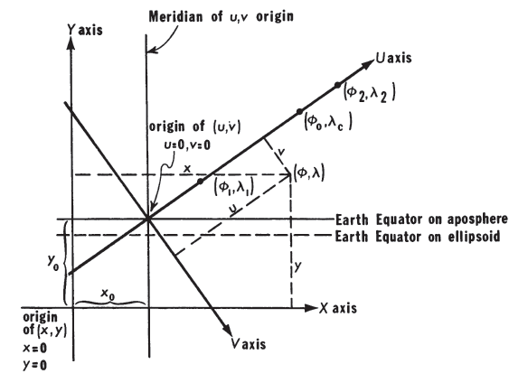
FIGURE 13.— Coordinate system for the Hotine Oblique Mercator projection
Equivalent to (9- 11):
Equivalent to (9- 12):
Alternate B. The following equations provide constants for the Hotine Oblique Mercator projection to fit a given central point and azimuth of the central line through the central point. Given: $a, e, k_0, \phi_0,$ and $(\phi,\lambda)$ as for alternate A, but instead of $(\phi_1, \lambda_1)$ and $(\phi_2, \lambda_2)$, $\lambda_c$ and $\alpha_c$ are given,
where
The inverse equations for the Hotine Oblique Mercator projection on the ellipsoid may be shown with few additional formulas. To determine $\phi$ and $\lambda$ from $x$ and $y$, or from $u$ and $v$, the same parameters of the map must be given, except for $\phi$ and $\lambda$, and the constants of the map are found from the above equations (9-11) through (9-24) for alternate A or (9-11) through (9-38) for alternate B. Then, if $x$ and $y$ are given in accordance with the definitions for the forward equations, they must first be converted to $(u, v)$:
To avoid the iteration, the series (3-5) may be used with (7-13) in place of (7-9):
The equivalent inverse equations as given by Hotine are as follows, following the calculation of constants using the same formulas as those given in his forward equations:
Hotine uses positive west longitude, x corresponding to u here, and y corresponding to -v here. Thomas uses positive west longitude, y corresponding to u here, and x corresponding to -v here. In calculations of Alaska zone 1, west longitude is positive, but u and v agree with u and v, respectively, here. ↩︎