Cylindrical Map Projections #
The map projection best known by name is certainly the Mercator - one of the cylindricals. Perhaps easiest to draw, if simple tables are on hand, the regular cylindrical projections consist of meridians which are equidistant parallel straight lines, crossed at right angles by straight parallel lines of latitude, generally not equidistant. Geometrically, cylindrical projections can be partially developed by unrolling a cylinder which has been wrapped around a globe representing the Earth, touching at the Equator, and on which meridians have been projected from the center of the globe (fig. 1). The latitudes can also be perspectively projected onto the cylinder for some projections (such as the Cylindrical Equal-Area and the Gall), but not on the Mercator and several others. When the cylinder is wrapped around the globe in a different direction, so that it is no longer tangent along the Equator, an oblique or transverse projection results, and neither the meridians nor the parallels will generally be straight lines.
7. MERCATOR PROJECTION #
SUMMARY #
- Cylindrical.
- Conformal.
- Meridians are equally spaced straight lines.
- Parallels are unequally spaced straight lines, closest near the Equator, cutting meridians at right angles.
- Scale is true along the Equator, or along two parallels equidistant from the Equator.
- Loxodromes (rhumb lines) are straight lines.
- Not perspective.
- Poles are at infinity; great distortion of area in polar regions.
- Used for navigation.
- Presented by Mercator in 1569.
HISTORY #
The well-known Mercator projection was perhaps the first projection to be regularly identified when atlases of over a century ago gradually began to name projections used, a practice now fairly commonplace. While the projection was apparently used by Erhard Etzlaub (1462-1532) of Nuremberg on a small map on the cover of some sundials constructed in 1511 and 1513, the principle remained obscure until Gerardus Mercator (1512-94) (fig. 7) independently developed it and presented it in 1569 on a large world map of 21 sections totaling about 1.3 by 2 m (Keuning, 1955, p. 17-18).
Mercator, born at Rupelmonde in Flanders, was probably originally named Gerhard Cremer (or Kremer), but he always used the latinized form. To his contemporaries and to later scholars, he is better known for his skills in map and globe making, for being the first to use the term “atlas” to describe a collection of maps in a volume, for his calligraphy, and for first naming North America as such on a map in 1538. To the world at large, his name is identified chiefly with his projection, which he specifically developed to aid navigation. His 1569 map is entitled “Nova et Aucta Orbis Terrae Descriptio ad Usum Navigantium Emendate Accommodata (A new and enlarged description of the Earth with corrections for use in navigation).” He described in Latin the nature of the projection in a large panel covering much of his portrayal of North America:
In this mapping of the world we have [desired] to spread out the surface of the globe into a plane that the places shall everywhere be properly located, not only with respect to their true direction and distance, one from another, but also in accordance with their due longitude and latitude; and further, that the shape of the lands, as they appear on the globe, shall be preserved as far as possible. For this there was needed a new arrangement and placing of meridians, so that they shall become parallels, for the maps hitherto produced by geographers are, on account of the curving and the bending of the meridians, unsuitable for navigation. Taking all this into consideration, we have somewhat increased the degrees of latitude toward each pole, in proportion to the increase of the parallels beyond the ratio they really have to the equator. (Fite and Freeman, 1926, p. 77-78.)
Mercator probably determined the spacing graphically, since tables of secants had not been invented. Edward Wright (ca. 1558-1615) of England later developed the mathematics of the projection and in 1599 published tables of cumulative secants, thereby indicating the spacing from the Equator (Keuning, 1955, p. 18). FIGURE 7.— Gerardus Mercator (1512-94). The inventor of the most famous map projection, which is the prototype for conformal mapping.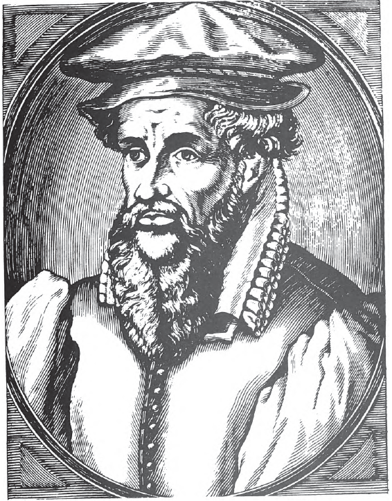
FEATURES AND USAGE #
The meridians of longitude of the Mercator projection are vertical parallel equally spaced lines, cut at right angles by horizontal straight parallels which are increasingly spaced toward each pole so that conformality exists (fig. 8). The spacing of parallels at a given latitude on the sphere is proportional to the secant of the latitude.
The major navigational feature of the projection is found in the fact that a sailing route between two points is shown as a straight line, if the direction or azimuth of the ship remains constant with respect to north. This kind of route is called a loxodrome or rhumb line and is usually longer than the great circle path (which is the shortest possible route on the sphere). It is the same length as a great circle only if it follows the Equator or a meridian. The projection has been standard since 1910 for nautical charts prepared by the former U.S. Coast and Geodetic Survey (now National Ocean Service) (Shalowitz, 1964, p. 302).
FIGURE 8.— The Mercator projection. The best-known projection. All angles are shown correctly, therefore, small shapes are essentially true, and it is called conformal. Since rhumb lines are shown straight on this projection, it is very useful in navigation. It is commonly used to show Equatorial regions of the Earth and other bodies.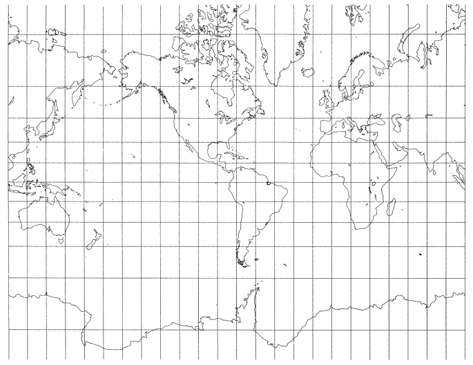
Nevertheless, the Mercator projection is fundamental in the development of map projections, especially those which are conformal. It remains a standard navigational tool. It is also especially suitable for conformal maps of equatorial regions. The USGS has recently used it as an inset of the Hawaiian Islands on the 1:500,000-scale base map of Hawaii, for a Bathymetric Map of the Northeast Equatorial Pacific Ocean (although the projection is not stated) and for a Tectonic Map of the Indonesia region, the latter two both in 1978 and at a scale of 1:5,000,000.
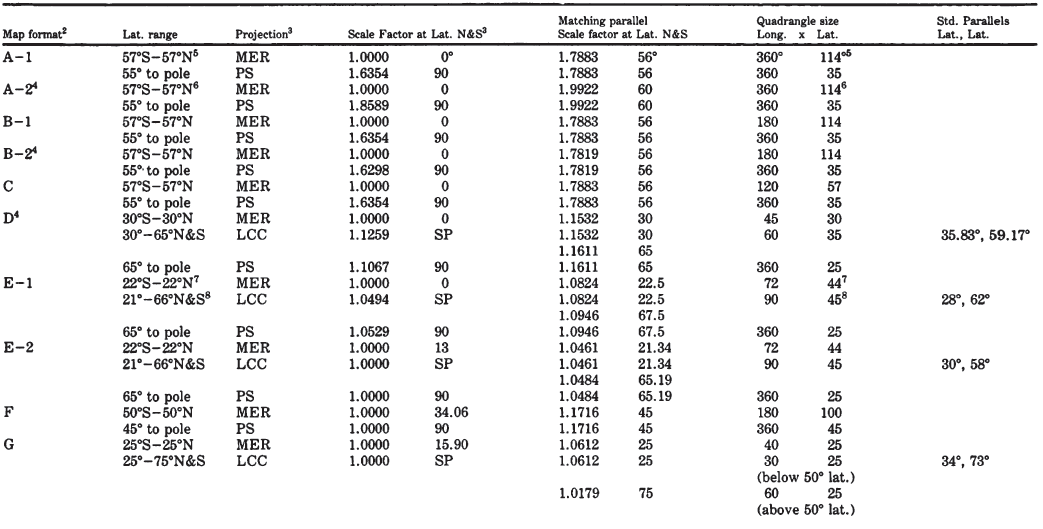
The first detailed map of an entire planet other than the Earth was issued in 1972 at a scale of 1:25,000,000 by the USGS Center of Astrogeology, Flagstaff, Arizona, following imaging of Mars by Mariner 9. Maps of Mars at other scales have followed. The mapping of the planet Mercury followed the flybys of Mariner 10 in 1974. Beginning in the late 1960’s, geology of the visible side of the Moon was mapped by the USGS in quadrangle fashion at a scale of 1:1,000,000. The four Galilean satellites of Jupiter and several satellites of Saturn were mapped following the Voyager missions of 1979-81. For all these bodies, the Mercator projection has been used to map equatorial portions, but coverage extended in some early cases to lats. 65" N. and S. (table 6).
TABLE 6.— Map projections used for extraterrestrial mapping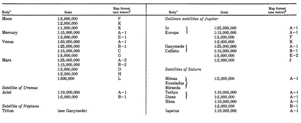
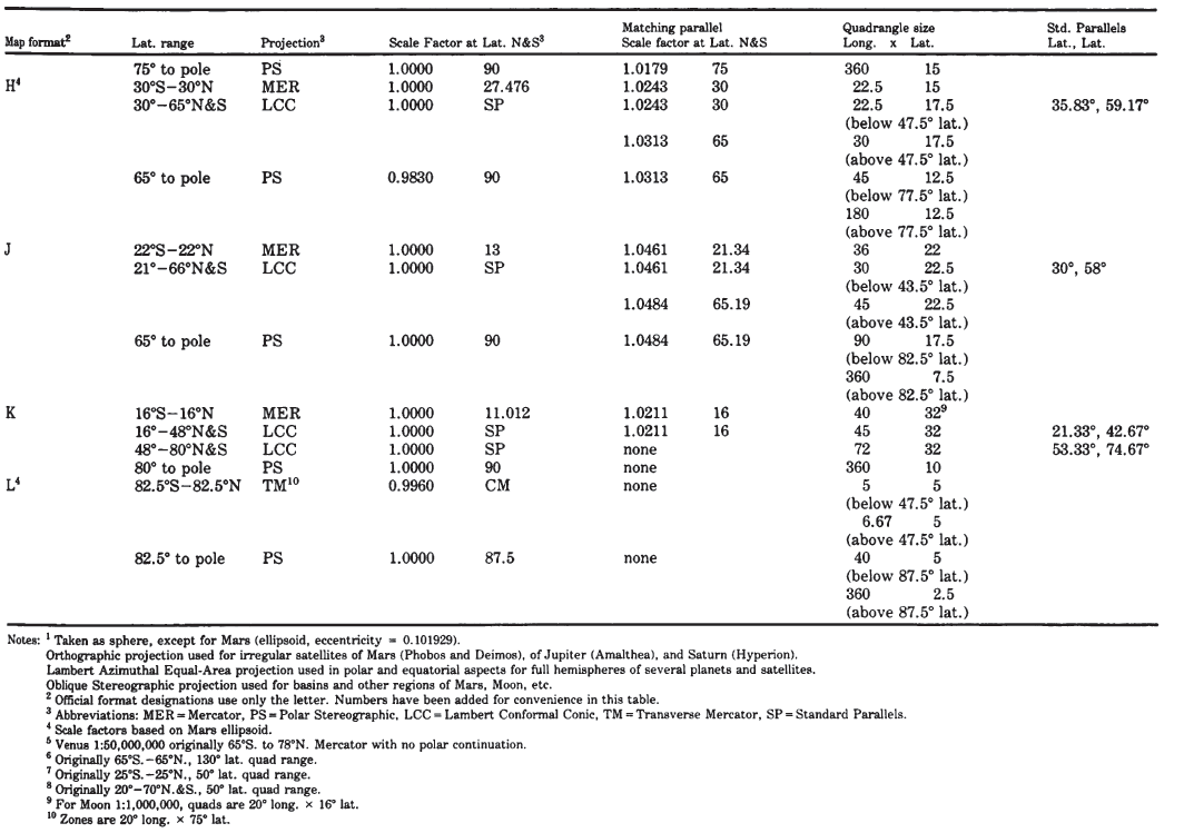
The cloudy atmosphere of Venus, circled by the Pioneer Venus Orbiter beginning in late 1978, is delaying more precise mapping of that planet, but the Mercator projection alone was used to show altitudes based on radar reflectivity over about 93 percent of the surface.
FORMULAS FOR THE SPHERE #
There is no suitable geometrical construction of the Mercator projection. For the sphere, the formulas for rectangular coordinates are as follows:
The inverse formulas for the sphere, to obtain $\phi$ and $\lambda$ from rectangular coordinates, are as follows:
FORMULAS FOR THE ELLIPSOID #
For the ellipsoid, the corresponding equations for the Mercator are only a little more involved (see numerical example):
The X and Y axes are oriented as they are for the spherical formulas, and $(\lambda-\lambda_0)$ should be similarly adjusted. Thomas also provides a series equivalent to equation (7-7), slightly modified here for consistency:
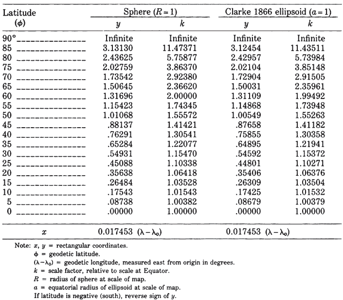
TABLE 7.— Mercator projection: Rectangular coordinates
It should be noted that $k$ for the sphere applies only to the sphere. The spherical projection is not conformal with respect to the ellipsoidal Earth, although the variation is negligible for a map with an equatorial scale of 1:15,000,000 or smaller. It should be noted that any central meridian can be chosen as $\lambda_0$ for an existing Mercator map, if forward or inverse formulas are to be used for conversions.
MEASUREMENT OF RHUMB LINES #
Since a major feature of the Mercator projection is the straight portrayal of rhumb lines, formulas are given below to determine their true lengths and azimuths. If a straight line on the map connects two points with respective latitudes and longitudes $(\phi_1, \lambda_1)$ and $(\phi_2, \lambda_2)$, the respective rectangular coordinates $(x_1, y_1)$ and $(x_2, y_2)$ are calculated using equations (7-1) and (7-2) for the sphere or (7-6) and (7-7) for the ellipsoid, inserting the respective subscripts.
For the true (not magnetic) compass bearing or azimuth $Az$ clockwise from north along the rhumb line,
For the true distance s along the rhumb line from $\phi_1$ to $\phi_2$,
where $M_2$ and $M_1$, the distances from the Equator along the meridian, are found for $\phi_2$ and $\phi_1$, respectively, using equation (3-21) and the same subscripts on $M$ and $\phi$:
MERCATOR PROJECTION WITH ANOTHER STANDARD PARALLEL #
The above formulas are based on making the Equator of the Earth true to scale on the map. Thus, the Equator may be called the standard parallel. It is also possible to have, instead, another parallel (actually two) as standard, with true scale. For the Mercator, the map will look exactly the same; only the scale will be different. If latitude $\phi_1$, is made standard (the opposite latitude $-\phi_1$ is also standard), the above forward formulas are adapted by multiplying the right side of equations (7-1) through (7-3) for the sphere, including the alternate forms, by $\cos\phi_1$. For the ellipsoid, the right sides of equations (7-6), (7-7), (7-8), and (7-7a) are multiplied by $\cos\phi_1/(1-e^2\sin^2\phi_1)^{1/2}$. For inverse equations, divide $x$ and $y$ by the same values before use in equations (7-4) and (7-5) or (7-10) and (7-12). Such a projection is most commonly used for a navigational map of part of an ocean, such as the North Atlantic Ocean, but the USGS has used it for equatorial quadrangles of some extraterrestrial bodies as described in table 6.
8. TRANSVERSE MERCATOR PROJECTION #
SUMMARY #
- Cylindrical (transverse).
- Conformal.
- Central meridian, each meridian 90" from central meridian, and Equator are straight lines.
- Other meridians and parallels are complex curves.
- Scale is true along central meridian, or along two straight lines equidistant from and parallel to central meridian. (These lines are only approximately straight for the ellipsoid.)
- Scale becomes infinite on sphere 90° from central meridian.
- Used extensively for quadrangle maps at scales from 1:24,000 to 1:250,000.
- Presented by Lambert in 1772.
HISTORY #
Since the regular Mercator projection has little error close to the Equator (the scale 10° away is only 1.5 percent larger than the scale at the Equator), it has been found very useful in the transverse form, with the equator of the projection rotated 90° to coincide with the desired central meridian. This is equivalent to wrapping the cylinder around a sphere or ellipsoid representing the Earth so that it touches the central meridian throughout its length, instead of following the Equator of the Earth. The central meridian can then be made true to scale, no matter how far north and south the map extends, and regions near it are mapped with low distortion. Like the regular Mercator, the map is conformal.
The Transverse Mercator projection in its spherical form was invented by the prolific Alsatian mathematician and cartographer Johann Heinrich Lambert (1728-77) (fig. 9). It was the third of seven new projections which he described in 1772 in his classic Beitrage (Lambert, 1772). At the same time, he also described what are now called the Cylindrical Equal-Area, the Lambert Conformal Conic, and the Lambert Azimuthal Equal-Area, each of which will be discussed subsequently; others are omitted here. He described the Transverse Mercator as a conformal adaptation of the Sinusoidal projection, then commonly in use (Lambert, 1772, p. 57-58). Lambert’s derivation was followed with a table of coordinates and a map of the Americas drawn according to the projection.
Little use has been made of the Transverse Mercator for single maps of continental areas. While Lambert only indirectly discussed its ellipsoidal form, mathematician Carl Friedrich Gauss (1777-1855) analyzed it further in 1822, and L. Krüger published studies in 1912 and 1919 providing formulas suitable for calculation relative to the ellipsoid. It is, therefore, sometimes called the Gauss Conformal or the Gauss-Krüger projection in Europe, but Transverse Mercator, a term first applied by the French map projection compiler Germain, is the name normally used in the United States (Thomas, 1952, p. 91-92; Germain, 1865?, p. 347).
Until recently, the Transverse Mercator projection was not precisely applied to the ellipsoid for the entire Earth. Ellipsoidal formulas were limited to series for relatively narrow bands. In 1945, E. H. Thompson (and in 1962, L. P. Lee) presented exact or closed formulas permitting calculation of coordinates for the full ellipsoid, although elliptic functions, and therefore lengthy series, numerical integrations, and (or) iterations, are involved (Lee, 1976, p. 92-101; Snyder, 1979a, p. 73; Dozier, 1980).
The formulas for the complete ellipsoid are interesting academically, but they are practical only within a band between 4° of longitude and some 10° to 15° of arc distance on either side of the central meridian, because of the much more significant scale errors fundamental to any projection covering a larger area. FIGURE 9.— Johann Heinrich Lambert (1728-77). Inventor of the Transverse Mercator, the Conformal Conic, the Azimuthal Equal-Area, and other important projections, as well as outstanding developments in mathematics, astronomy, and physics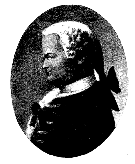
FEATURES #
The meridians and parallels of the Transverse Mercator (fig. 10) are no longer the straight lines they are on the regular Mercator, except for the Earth’s Equator, the central meridian, and each meridian 90° away from the central meridian. Other meridians and parallels are complex curves.
The spherical form is conformal, as is the parent projection, and scale error is only a function of the distance from the central meridian, just as it is only a function of the distance from the Equator on the regular Mercator. The ellipsoidal form is also exactly conformal, but its scale error is slightly affected by factors other than the distance alone from the central meridian (Lee, 1976, p. 98). FIGURE 10.— The Transverse Mercator projection. While the regular Mercator has constant scale along the Equator, the Transverse Mercator has constant scale along any chosen central meridian. This projection is conformal and is often used to show regions with greater north-south extent.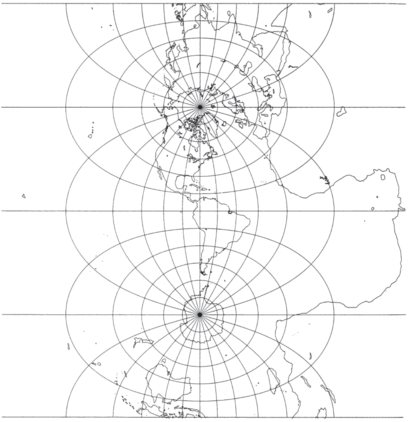
With the scale along the central meridian remaining constant, the Transverse Mercator is an excellent projection for lands extending predominantly north and south.
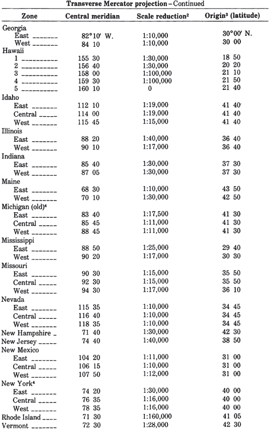
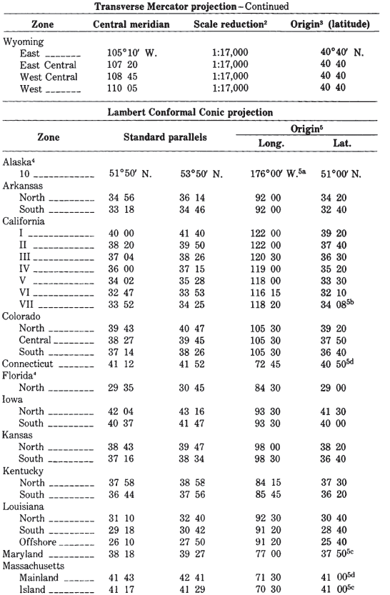
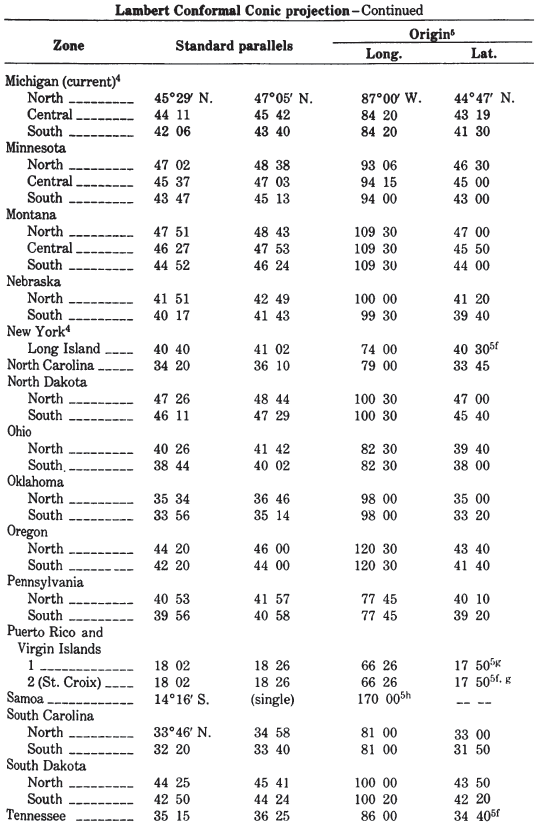
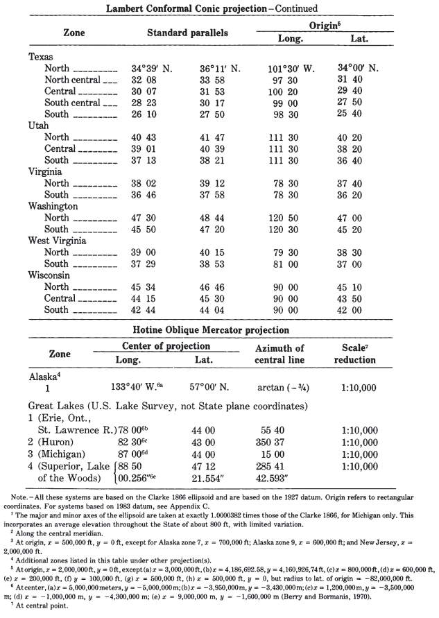
TABLE 8.— U.S. State plane coordinate systems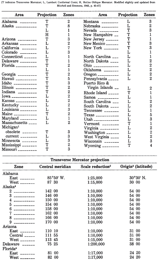
USAGE #
The Transverse Mercator projection (spherical or ellipsoidal) was not described by Close and Clarke in their generally detailed article in the 1911 Encyclopaedia Britannica because it was “seldom used” (Close and Clarke, 1911, p. 663). Deetz and Adams (1934) favorably referred to it several times, but as a slightly used projection.
The spherical form of the Transverse Mercator has been used by the USGS only recently. In 1979, this projection was chosen for a base map of North America at a scale of 1:5,000,000 to replace the Bipolar Oblique Conic Conformal projection previously used for tectonic and other geologic maps. The scale factor along the central meridian, long. 100° W., is reduced to 0.926. The radius of the Earth is taken at 6,371,204 m, with approximately the same surface area as the International ellipsoid, placing the two straight lines of true design scale 2,343 km on each side of the central meridian.
While its use in the spherical form is limited, the ellipsoidal form of the Transverse Mercator is probably used more than any other one projection for geodetic mapping.
In the United States, it is the projection used in the State Plane Coordinate System (SPCS) for States with predominant north-south extent. (The Lambert Conformal Conic is used for the others, except for the panhandle of Alaska, which is prepared on the Oblique Mercator. Alaska, Florida, and New York use both the Transverse Mercator and the Lambert Conformal Conic for different zones.) Except for narrow States, such as Delaware, New Hampshire, and New Jersey, all States using the Transverse Mercator are divided into two to eight zones, each with its own central meridian, along which the scale is slightly reduced to balance the scale throughout the map. Each zone is designed to maintain scale distortion within 1 part in 10,000. Several States beginning in 1935 also passed legislation establishing the SPCS as a permissible system for recording boundary descriptions or point locations. Several zone changes have occurred for use with the new 1983 datum. They are listed in Appendix C.
In addition to latitude and longitude as the basic frame of reference, the corresponding rectangular grid coordinates in feet are used to designate locations (Mitchell and Simmons, 1945). The parameters for each State are given in table 8. All are based on the Clarke 1866 ellipsoid. It is important to note that, for the metric conversion to feet using this coordinate system, 1 m equals exactly 39.37in., not the current standard accepted by the National Bureau of Standards in 1959, in which 1 in. equals exactly 2.54 cm. Surveyors continue to follow the former conversion for consistency. The difference is only two parts in a million, but it is enough to cause confusion, if it is not accounted for.
Beginning with the late 1950’s, the Transverse Mercator projection was used by the USGS for nearly all new quadrangles (maps normally bounded by meridians and parallels) covering those States using the TM Plane Coordinates, but the central meridian and scale factor are those of the SPCS zone. Thus, all quadrangles for a given zone may be mosaicked exactly. Beginning in 1977, many USGS maps have been produced on the Universal Transverse Mercator projection (see below). Prior to the late 1950’s, the Polyconic projection was used. The change in projection was facilitated by the use of high-precision rectangular-coordinate plotting machines. Some maps produced on the Transverse Mercator projection system during this transition period are identified as being prepared according to the Polyconic projection. Since most quadrangles cover only 7½ minutes (at a scale of 1:24,000) or 15 minutes (at 1:62,500) of latitude and longitude, the difference between the Polyconic and the Transverse Mercator for such a small area is much more significant due to the change of central meridian than due to the change of projection. The difference is still slight and is detailed later under the discussion of the Polyconic projection. The Transverse Mercator is used in many other countries for official topographic mapping as well. The Ordnance Survey of Great Britain began switching from a Transverse Equidistant Cylindrical (the Cassini-Soldner) to the Transverse Mercator about 1920.
The use of the Transverse Mercator for quadrangle maps has been recently extended by the USGS to include the planet Mars. Although other projections are used at smaller scales, quadrangles at scales of 1:1,000,000 and 1:250,000, and covering areas from 200 to 800 km on a side, were drawn to the ellipsoidal Transverse Mercator between lats. 65°N. and S. The scale factor along the central meridian was made 1.0. For the current series, see table 6.
In addition to its own series of larger-scale quadrangle maps, the Army Map Service used the Transverse Mercator for two other major mapping operations:
(1) a series of 1:250,000-scale quadrangle maps covering the entire country, and
(2) as the geometric basis for the Universal Transverse Mercator (UTM) grid.
The entire area of the United States has been mapped since the 1940’s in sections 2° of longitude (between even-numbered meridians, but in 3° sections in Alaska) by 1° of latitude (between each full degree) at a scale of 1:250,000, with the UTM grid superimposed and with some variations in map boundaries at coastlines. These maps were drawn with reference to their own central meridians, not the central meridians of the UTM zones (see below), although the 0.9996 central scale factor was employed. The central meridian of about one-third of the maps coincides with the central meridian of the zone, but it does not for about two-thirds, the “wing” sheets, which therefore do not perfectly match the center sheets. The USGS has assumed publication and revision of this series and is casting new maps using the correct central meridians.
Transverse Mercator quadrangle maps fit continuously in a north-south direction, provided they are prepared at the same scale, with the same central meridian, and for the same ellipsoid. They do not fit exactly from east to west, if they have their own central meridians; although quadrangles and other maps properly constructed at the same scale, using the SPCS or UTM projection, fit in all directions within the same zone.
UNIVERSAL TRANSVERSE MERCATOR PROJECTION #
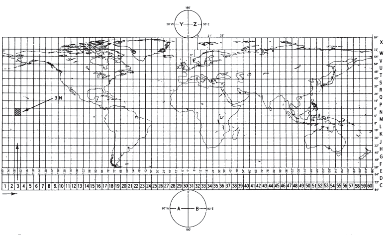
The Universal Transverse Mercator (UTM) projection and grid were adopted by the U.S. Army in 1947 for designating rectangular coordinates on large-scale military maps of the entire world. The UTM is the ellipsoidal Transverse Mercator to which specific parameters, such as central meridians, have been applied. The Earth, between lats. 84° N. and 80° S., is divided into 60 zones each generally 6° wide in longitude. Bounding meridians are evenly divisible by 6°, and zones are numbered from 1 to 60 proceeding east from the 180th meridian from Greenwich with minor exceptions. There are letter designations from south to north (see fig. 11). Thus, Washington, D.C., is in grid zone 18S, a designation covering a quadrangle from long. 72° to 78° W. and from lat. 32° to 40deg; N. Each of these quadrangles is further subdivided into grid squares 100,000 meters on a side with double-letter designations, including partial squares at the grid boundaries. From lat. 84° N. and 80° S. to the respective poles, the Universal Polar Stereographic (UPS) projection is used instead.
As with the SPCS, each geographic location in the UTM projection is given $x$ and $y$ coordinates, but in meters, not feet, according to the Transverse Mercator projection, using the meridian halfway between the two bounding meridians as the central meridian, and reducing its scale to 0.9996 of true scale (a 1:2,500 reduction). The reduction was chosen to minimize scale variation in a given zone; the variation reaches 1 part in 1,000 from true scale at the Equator. The USGS, for civilian mapping, uses only the zone number and the $x$ and $y$ coordinates, which are sufficient to define a point, if the ellipsoid and the hemisphere (north or south) are known; the 100,000-m square identification is not essential. The lines of true scale are approximately parallel to and approximately 180 km east and west of the central meridian. Between them, the scale is too small; beyond them, it is too great. In the Northern Hemisphere, the Equator at the central meridian is considered the origin, with an $x$ coordinate of 500,000 m and a $y$ of 0. For the Southern Hemisphere, the same point is the origin, but, while $x$ remains 500,000 m, $y$ is 10,000,000 m. In each case, numbers increase toward the east and north. Negative coordinates are thus avoided (Army, 1973, p. 7, endmap). A page of coordinates for the UTM projection is shown in table 9. TABLE 9.— Universal Transverse Mercator grid coordinates FIGURE 11.— Universal Transverse Mercator (UTM) grid zone designations for the world shown on a horizontally expanded Equidistant Cylindrical projection index map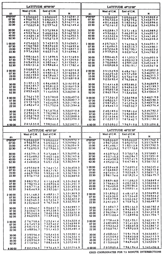
The ellipsoidal Earth is used throughout the UTM projection system, but the reference ellipsoid changes with the particular region of the Earth. For all land under United States jurisdiction, the Clarke 1866 ellipsoid is used for the map projection. For the UTM grid superimposed on the map of Hawaii, however, the International ellipsoid is used. The Geological Survey uses the UTM graticule and grid for its 1:250,000- and larger-scale maps of Alaska, and applies the UTM grid lines or tick marks to its quadrangles and State base maps for the other States, although they are generally drawn with different projections or parameters.
FORMULAS FOR THE SPHERE #
A partially geometric construction of the Transverse Mercator for the sphere involves constructing a regular Mercator projection and using a transforming map to convert meridians and parallels on one sphere to equivalent meridians and parallels on a sphere rotated to place the equator of one along the chosen central meridian of the other. Such a transforming map may be the equatorial aspect of the Stereographic or other azimuthal projection, drawn twice to the same scale on transparencies. The transparencies may then be superimposed at 90° angles and the points compared.
In an age of computers, it is much more satisfactory to use mathematical formulas. The rectangular coordinates for the Transverse Mercator applied to the sphere (Thomas, 1952, p. 6):
The inverse formulas for$(\phi,\lambda)$ in terms of $(x,y)$:
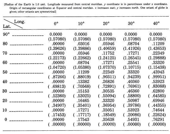
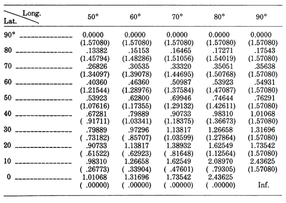
TABLE 10.— Transverse Mercator projection: Rectangular coordinates for the sphere
FORMULAS FOR THE ELLIPSOID #
For the ellipsoidal form, the most practical form of the equations is a set of series approximations which converge rapidly to the correct centimeter or less at full scale in a zone extending 3° to 4° of longitude from the central meridian. Beyond this, the forward series as given here is accurate to about a centimeter at 7° longitude, but the inverse series does not have sufficient terms for this accuracy. The forward series may be used with meter accuracy to 10° of longitude. (Many additional terms for use to 24° of longitude may be found in Army (1962).) Coordinate axes are the same as they are for the spherical formulas above. The formulas below are only slightly modified from those presented in standard references to provide mm accuracy at full scale (Army, 1973, p. 5-7; Thomas, 1952, p. 2-3). (See numerical examples)
$M_0 = M$ calculated for $\phi_0$ the latitude crossing the central meridian $\lambda_0$ at the origin of the $x, y$ coordinates. Note: If $\phi=\pm\pi/2$, all equations should be omitted except (3-21), from which $M$ and $M_0$ are calculated. Then $x=0, y=k_0(M-M_0), k=k_0$.
Equation (8-11) for $k$ may also be written as a function of $x$ and $\phi$:
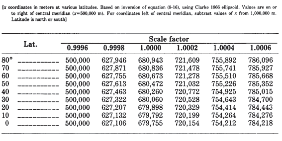
TABLE 11.— Universal Transverse Mercator projection: Location of points with given scale factor
To obtain UTM or SPCS coordinates, the appropriate “false easting” is added to $x$ and “false northing” added to $y$ after calculation using (8-9) and (8-10).
For the inverse formulas (Army, 1973, p. 6, 7, 46; Thomas, 1952, p. 2-3):
It may be found from equation (3-26):
For improved computational efficiency using series (3-21) and (3-26), see p. 19. From $\phi_1$, other terms below are calculated for use in equations (8-17) and (8-18). (If $\phi_1 = \pm\pi/2$, (8-12), (8-21) through (8-25), (8-17) and (8-18) are omitted, but $\phi=\pm90°$ taking the sign of $y$, while $\lambda$ is indeterminate, and may be called $\lambda_0$. Also, $k = k_0$.)
“MODIFIED TRANSVERSE MERCATOR” PROJECTION #
In 1972, the USGS devised a projection specifically for the revision of a 1954 map of Alaska which, like its predecessors, was based on the Polyconic projection. The projection was drawn to a scale of 1:2,000,000 and published at 1:2,500,000 (map “E”) and 1:1,584,000 (map “B”). Graphically prepared by adapting coordinates for the Universal Transverse Mercator projection, it is identified as the “Modified Transverse Mercator” projection. It resembles the Transverse Mercator in a very limited manner and cannot be considered a cylindrical projection. It approximates an Equidistant Conic projection for the ellipsoid in actual construction. Because of the projection name, it is listed here. The projection was also used in 1974 for a base map of the Aleutian-Bering Sea Region published at the 1:2,500,000 scale.
The basis for the name is clear from an unpublished 1972 description of the projection, in which it is also stressed that the “latitudinal lines are parallel” and the “longitudinal lines are straight.” The computations
were taken from the AMS Technical Manual #21 (Universal Transverse Mercator) based on the Clarke 1866 Spheroid.*** The projection was started from a N-S central construction line of the 153° longitude which is also the centerline of Zone 5 from the UTM tables. Along this line each even degree latitude was plotted from book values. At the plotted point for the 64° latitude, a perpendicular to the construction line (153°) was plotted. From the center construction line for each degree east and west for 4° (the limits of book value of Zone #5) the curvature of latitude was plotted. From this 64° latitude, each 2° latitude north to 70° and south to 54° was constructed parallel to the 64° latitude line. Each degree of longitude was plotted on the 58° and 68° latitude line. Through corresponding degrees of longitude along these two lines of latitude a straight line (line of longitude) was constructed and projected to the limits of the map. This gave a small projection 8° in width and approximately 18° in length. This projection was repeated east and west until a projection of some 72° in width was attained.
For transferring data to and from the Alaska maps, it was necessary to determine projection formulas for computer programming. Since it appeared to be unnecessarily complicated to derive formulas based on the above construction, it was decided to test empirical formulas with actual coordinates. After careful measurements of coordinates for graticule intersections were made in 1979 on the stable-base map, it was determined that the parallels very closely approximate concentric circular arcs, spaced in proportion to their true distances on the ellipsoid, while the meridians are nearly equidistant straight lines radiating from the center of the circular arcs. Two parallels have a scale equal to that along the meridians. The Equidistant Conic projection for the ellipsoid with two standard parallels was then applied to these coordinates as the closest approximation among projections with available formulas. After various trial values for scale and standard parallels were tested, the empirical formulas below (equations (8-26) through (8-32)) were obtained. These agree with measured values within 0.005 inch at mapping scale for 44 out of 58 measurements made on the map and within 0.01 inch for 54 of them.
FORMULAS FOR THE “MODIFIED TRANSVERSE MERCATOR” PROJECTION #
The “Modified Transverse Mercator” projection was found to be most closely equivalent to an Equidistant Conic projection for the Clarke 1866 ellipsoid, with the scale along the meridians reduced to 0.9992 of true scale and the standard parallels at lat. 66.09° and 53.50° N. (also at 0.9992 scale factor). For the Alaska Map “E” at 1:2,500,000, using long. 150° W. as the central meridian and lat. 58° N. as the latitude of the origin on the central meridian, the general formulas (Snyder, 1978a, p. 378) reduce with the above parameters to the following, giving x and y in meters at the map scale. The Y axis lies along the central meridian, y increasing northerly, and the X axis is perpendicular at the origin, x increasing easterly.
The equation for $\phi$, (8-31), involves iteration by successive substitution. If an initial $\phi$ of 60° is inserted into the right side, $\phi$ on the left may be calculated and substituted into the right in place of the previous trial $\phi$. Recalculations continue until the change in $\phi$ is less than a preset convergence. If $\lambda$ as calculated is less than -180°, it should be added to 360° and labeled East Longitude.
Formulas to adjust $x$ and $y$ for the map inset of the Aleutian Islands are omitted here, but the coordinates above are rotated counterclockwise 29.79° and transposed to + 0.798982 m for x and + 0.347600 m for y.
9. OBLIQUE MERCATOR PROJECTION #
SUMMARY #
- Cylindrical (oblique).
- Conformal.
- Two meridians 180° apart are straight lines.
- Other meridians and parallels are complex curves.
- Scale on the spherical form is true along chosen central line, a great circle at an oblique angle, or along two straight lines parallel to central line. The scale on the ellipsoidal form is similar, but varies slightly from this pattern.
- Scale becomes infinite 90° from the central line.
- Used for grids on maps of the Alaska panhandle, for mapping in Switzerland, Madagascar, and Borneo and for atlas maps of areas with greater extent in an oblique direction.
- Developed 1900-50 by Rosenmund, Laborde, Hotine, and others.
HISTORY #
There are several geographical regions such as the Alaska panhandle centered along lines which are neither meridians nor parallels, but which may be taken as great circle routes passing through the region. If conformality is desired in such cases, the Oblique Mercator is a projection which should be considered.
The historical origin of the Oblique Mercator projection does not appear to be sharply defined, although it is a logical generalization of the regular and Transverse Mercator projections. Apparently, Rosenmund (1903) made the earliest published reference, when he devised an ellipsoidal form which is used for topographic mapping of Switzerland. The projection was not mentioned in the detailed article on “Map Projections” in the 1911 Encyclopaedia Britannica (Close and Clarke, 1911) or in Hinks’ brief text (1912). Laborde applied the Oblique Mercator to the ellipsoid for the topographic mapping of Madagascar in 1928 (Young, 1930; Laborde, 1928). H. J. Andrews (1935, 1938) proposed the spherical forms for maps of the United States and Eurasia. Hinks presented seven world maps on the Oblique Mercator, with poles located in several different positions, and a consequent variety in the regions shown more satisfactorily (Hinks, 1940, 1941).
A study of conformal projections of the ellipsoid by British geodesist Martin Hotine (1898-1968), published in 1946-47, is the basis of the U.S. use of the ellipsoidal Oblique Mercator, which Hotine called the “rectified skew orthomorphic” (Hotine, 1947, p. 66-67). The Hotine approach has limitations, as discussed below, but it provides closed formulas which have been adapted for U. S. mapping of suitable zones. One of its limitations is overcome by a recent series form of the ellipsoidal Oblique Mercator (Snyder, 1979a, p. 74), but other limitations result instead. This later form resulted from development of formulas for the continuous mapping of satellite images, using the Space Oblique Mercator projection (to be discussed later).
While Hotine projected the ellipsoid conformally onto an “aposphere” of constant total curvature and thence to a plane, J. H. Cole (1943, p. 16-30) projected the ellipsoid onto a “conformal sphere,” using conformal latitudes (described earlier) to make the sphere conformal with respect to the ellipsoid, then plotted the spherical Oblique Mercator from this intermediate sphere. Rosenmund’s system for Switzerland is a more complex double projection through a conformal sphere
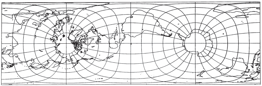
(Rosenmund, 1903; Bolliger, 1967). Laborde combined the conformal sphere with a complex-algebra transformation of the Oblique Mercator (Reignier, 1957, p. 130). FIGURE 12.— Oblique Mercator projection with the center of projection at lat. 45° N. on the central meridian. A straight line through the point and, in this example, perpendicular to the central meridian is true to scale. The projection is conformal and has been used for regions lying along a line oblique to meridians.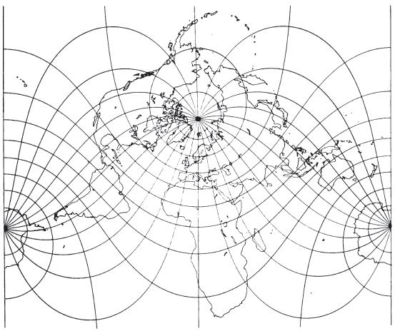
FEATURES #
The Oblique Mercator for the sphere is equivalent to a regular Mercator projection which has been altered by wrapping a cylinder around the sphere so that it touches the surface along the great circle path chosen for the central line, instead of along the Earth’s Equator. A set of transformed meridians and parallels relative to the great circle may be plotted bearing the same relationship to the rectangular coordinates for the Oblique Mercator projection, as the geographic meridians and parallels bear to the regular Mercator. It is, therefore, possible to convert the geographic meridians and parallels to the transformed values and then to use the regular Mercator equations, substituting the transformed values in place of the geographic values. This is the procedure for the sphere, although combined formulas are given below, but it becomes much more complicated for the ellipsoid. The advent of present-day computers and programmable pocket calculators make these calculations feasible for sphere or ellipsoid.
The resulting Oblique Mercator map of the world (fig. 12) thus resembles the regular Mercator with the landmasses rotated so that the poles and Equator are no longer in their usual positions. Instead, two points 90° away from the chosen great circle path through the center of the map are at infinite distance off the map. Normally, the Oblique Mercator is used only to show the region near the central line and for a relatively short portion of the central line. Under these conditions, it looks similar to maps of the same area using other projections, except that careful scale measurements will show differences.
It should be remembered that the regular Mercator is in fact a limiting form of the Oblique Mercator with the Equator as the central line, while the Transverse Mercator is another limiting form of the Oblique with a meridian as the central line. As with these limiting forms, the scale along the central line of the Oblique Mercator may be reduced to balance the scale throughout the map.
USAGE #
The Oblique Mercator projection is used in the spherical form for a few atlas maps. For example, the National Geographic Society uses it for atlas and sheet maps of Hawaii, the West Indies, and New Zealand. The spherical form is being used by the USGS for maps of North and South America and Australasia in a new set of 1:10,000,000-scale maps of Hydrocarbon Provinces. For North America, the central scale factor is 0.968, and the transformed pole is at lat. 10°N, long. 10°E. For South America, these numbers are 0.974, 10°N., and 30°E., respectively; for Australasia, 0.978, 55°N, and 160°W. These parameters were chosen after a least-squares analysis of over 100 points on each continent to determine optimum parameters for a common conformal projection.
In the ellipsoidal form it was used, as mentioned above, by Rosenmund for Switzerland and Laborde for Madagascar. Hotine used it for Malaya and Borneo and Cole for Italy. It is used in the Hotine form by the USGS for grid marks on zone 1 (the panhandle) of Alaska, using the State Plane Coordinate System as adapted to this projection by Erwin Schmid of the former Coast and Geodetic Survey. The Hotine form was also adopted by the U.S. Lake Survey for mapping of the five Great Lakes, the St. Lawrence River, and the U.S.-Canada Border Lakes west to the Lake of the Woods (Berry and Bormanis, 1970). Four zones are involved; see table 8 for parameters of these and the Alaska zones. TABLE 12.— Hotine Oblique Mercator projection parameters used for Landsat 1, 2, and 3 imagery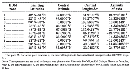
More recently, the Hotine form was adapted by John B. Rowland (USGS) for mapping Landsat 1, 2, and 3 satellite imagery in two sets of five discontinuous zones from north to south (table 12). The central line of the latter is only a close approximation to the satellite groundtrack, which does not follow a great circle route on the Earth; instead, it follows a path of constantly changing curvature. Until the mathematical implementation of the Space Oblique Mercator (SOM) projection, the Hotine Oblique Mercator (HOM) was probably the most suitable projection available for mapping Landsat type data. In addition to Landsat, the HOM projection has been used to cast Heat Capacity Mapping Mission (HCMM) imagery since 1978. NOAA (National Oceanic and Atmospheric Administration) has also cast some weather satellite imagery on the HOM to make it compatible with Landsat in the polar regions which are beyond Landsat coverage (above lat. 82°).
The parameters for a given map according to the Oblique Mercator projection may be selected in various ways. If the projection is to be used for the map of a smaller region, two points located near the limits of the region may be selected to lie upon the central line, and various constants may be calculated from the latitude and longitude of each of the two points. A second approach is to choose a central point for the map and an azimuth for the central line, which is made to pass through the central point. A third approach, more applicable to the map of a large portion of the Earth’s surface, treated as spherical, is to choose a location on the original sphere of the pole for a transformed sphere with the central line as the equator. Formulas are given for each of these approaches, for sphere and ellipsoid.
FORMULAS FOR THE SPHERE #
Starting with the forward equations, for rectangular coordinates in terms of latitude and longitude (see numerical examples):
Given two points to lie upon the central line, with latitudes and longitudes $(\phi_1,\lambda_1)$ and $(\phi_2,\lambda_2)$ and longitude increasing easterly and relative to Greenwich. The pole of the oblique transformation at $(\phi_p,\lambda_p)$ may be calculated as follows:
$$ \begin{align} \lambda_p = &\arctan[(\cos\phi_1\sin\phi_2\cos\lambda_1 - \sin\phi_1\cos\phi_2\cos\lambda_2)/ \\ &(\sin\phi_1\cos\phi_2\sin\lambda_2 - \cos\phi_1\sin\phi_2\sin\lambda_1)] \end{align} \tag{ 9-1 } $$$$ \phi_p = \arctan[-\cos(\lambda_p-\lambda_1)/\tan\phi_1] \tag{ 9-2 } $$The Fortran ATAN2 function or its equivalent should be used with equation (9-1), but not with (9-2). The other pole is located at $(-\phi_p,\lambda_p\pm\pi)$. Using the positive (northern) value of $\phi_p$, the following formulas give the rectangular coordinates for point $(\phi,\lambda)$, with $k_0$, the scale factor along the central line:$$ x = Rk_0\arctan\{[\tan\phi\cos\phi_p+\sin\phi_p\sin(\lambda-\lambda_0)]/\cos(\lambda-\lambda_0)\} \tag{ 9-3 } $$$$ y = (R/2)k_0\ln[(1+A)/(1-A)] \tag{ 9-4 } $$or$$ y=Rk_0\mathrm{arctanh}A \tag{ 9-4a } $$$$ k=k_0/(1-A^2)^{1/2} \tag{ 9-5 } $$where$$ A=\sin\phi_p\sin\phi - \cos\phi_p\cos\phi\sin(\lambda-\lambda_0) \tag{ 9-6 } $$With these formulas, the origin of rectangular coordinates lies at$$ \begin{align} \phi_0 &= 0 \\ \lambda_0 &=\lambda_p + \pi/2 \end{align} \tag{ 9-6a } $$and the X axis lies along the central line, $x$ increasing easterly. The transformed poles are $y$ equals infinity.Given a central point $(\phi_c,\lambda_c)$ with longitude increasing easterly and relative to Greenwich, and azimuth $\beta$ east of north of the central line through $(\phi_c,\lambda_c)$, the pole of the oblique transformation at $(\phi_p,\lambda_p)$ may be calculated as follows:
$$ \phi_p = \arcsin(\cos\phi_c\sin\beta) \tag{ 9-7 } $$$$ \lambda_p = \arctan[-\cos\beta/(-\sin\phi_c\sin\beta)]+ \lambda_c \tag{ 9-8 } $$These values of $\phi_p$ and $\lambda_p$, may then be used in equations (9-3) through (9-6) as before.For an extensive map, $\phi_p$ and $\lambda_p$ may be arbitrarily chosen by eye to give the pole for a central line passing through a desired portion of the globe. These values may then be directly used in equations (9-3) through (9-6) without intermediate calculation.
For the inverse formulas, equations (9-1) and (9-2) or (9-7) and (9-8) must first be used to establish the pole of the oblique transformation, if it is not known already. Then,
FORMULAS FOR THE ELLIPSOID #
These are the formulas provided by Hotine, slightly altered to use a positive eastern longitude (he used positive western longitude), to simplify calculations of hyperbolic functions, and to use symbols consistent with those of this bulletin. The central line is a geodesic, or the shortest route on an ellipsoid, corresponding to a great circle route on the sphere.
It is customary to provide rectangular coordinates for the Hotine in terms either of $(u, v)$ or $(x, y)$. The $(u, v)$ coordinates are similar in concept to the $(x, y)$ calculated for the foregoing spherical formulas, with $u$ corresponding to $x$ for the spherical formulas, increasing easterly from the origin along the central line, but $v$ corresponds to $-y$ for the spherical formulas, so that $v$ increases southerly in a direction perpendicular to the central line. For the Hotine, $x$ and $y$ are calculated from $(u, v)$ as “rectified” coordinates with the Y axis following the meridian passing through the center point, and increasing northerly as usual, while the X axis lies east and west through the same point. The X and Y axes thus lie in directions like those of the Transverse Mercator, but the scale-factor relationships remain those of the Oblique Mercator.
The normal origin for $(u, v)$ coordinates in the Hotine Oblique Mercator is approximately at the intersection of the central line wilh the Earth’s Equator. Actually it occurs at the crossing of the central line with the equator of the “aposphere,” and is, thus, a rather academic location. The “aposphere” is a surface with a constant “total” curvature based on the curvature along the meridian and perpendicular thereto on the ellipsoid at the chosen central point for the projection. The ellipsoid is conformally projected onto this aposphere, then to a plane. As a result, the Hotine is perfectly conformal, but the scale along the central line is true only at the chosen central point along that line or along a relatively flat elliptically shaped line approximately centered on that point, if the scale of the central point is arbitrarily reduced to balance scale over the map. The variation in scale along the central line is extremely small for a map extending less than 45° in arc, which includes most existing usage of the Hotine. A longer central line suggests the use of a different set of formulas, available as a limiting form of the Space Oblique Mercator projection. On Rosenmund’s (1903), Laborde’s (1928), and Cole’s (1943) versions of the ellipsoidal Oblique Mercator, the central line is a great circle arc on the intermediate conformal sphere, not a geodesic. As on Hotine’s version, this central line is not quite true to scale except at one or two chosen points.
The projection constants may be established for the Hotine in one of two ways, as they were for the spherical form. Two desired points, widely separated on the map, may be made to fall on the central line of the projection, or the central line may be given a desired azimuth through a selected central point. Taking these approaches in order:
Alternate A, with the central line passing through two given points.
Given:
- $a$ and $e$ for the reference ellipsoid
- $k_0 = $scale factor at the selected center of the map, lying on the central line.
- $\phi_0 = $latitude of selected center of the map.
- $(\phi_1,\lambda_1) = $latitude and longitude (east of Greenwich is positive) of the first point which is to lie on the central line.
- $(\phi_2,\lambda_2) = $latitude and longitude of the second point which is to lie on the central line.
- $(\phi,\lambda_) = $latitude and longitude of the point for which the coordinates are desired.
It is also necessary to place both $(\phi_1,\lambda_1)$ and $(\phi_2,\lambda_2)$ on the ascending portion, or both on the descending portion, of the central line, relative to the Earth’s Equator. That is, the central line should not pass through a maximum or minimum between these two points.
If $e$ is zero, the Hotine formulas give coordinates for the spherical Oblique Mercator.
Because of the involved nature of the Hotine formulas, they are given here in an order suitable for calculation, and in a form eliminating the use of hyperbolic functions as given by Hotine in favor of single calculations of exponential functions to save computer time. The corresponding Hotine equations are given later for comparison (see p. 274 for numerical examples).
Care should be taken that $(\lambda-\lambda_0)$ has 360° added or subtracted, if the 180th meridian falls between, since multiplication by $B$ eliminates automatic correction with the sin or cos function.
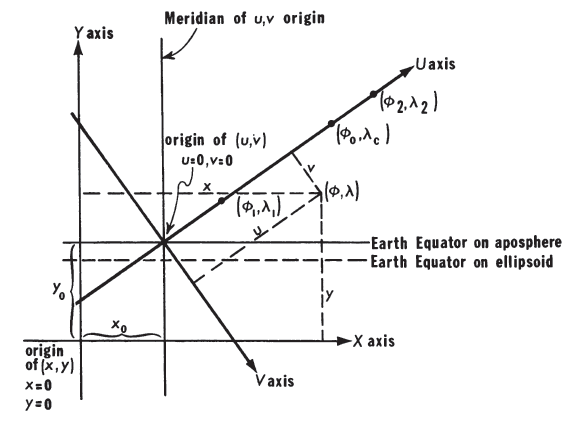
FIGURE 13.— Coordinate system for the Hotine Oblique Mercator projection
Equivalent to (9- 11):
Equivalent to (9- 12):
Alternate B. The following equations provide constants for the Hotine Oblique Mercator projection to fit a given central point and azimuth of the central line through the central point. Given: $a, e, k_0, \phi_0,$ and $(\phi,\lambda)$ as for alternate A, but instead of $(\phi_1, \lambda_1)$ and $(\phi_2, \lambda_2)$, $\lambda_c$ and $\alpha_c$ are given,
where
The inverse equations for the Hotine Oblique Mercator projection on the ellipsoid may be shown with few additional formulas. To determine $\phi$ and $\lambda$ from $x$ and $y$, or from $u$ and $v$, the same parameters of the map must be given, except for $\phi$ and $\lambda$, and the constants of the map are found from the above equations (9-11) through (9-24) for alternate A or (9-11) through (9-38) for alternate B. Then, if $x$ and $y$ are given in accordance with the definitions for the forward equations, they must first be converted to $(u, v)$:
To avoid the iteration, the series (3-5) may be used with (7-13) in place of (7-9):
The equivalent inverse equations as given by Hotine are as follows, following the calculation of constants using the same formulas as those given in his forward equations:
10. CYLINDRICAL EQUAL-AREA PROJECTION #
SUMMARY #
- Cylindrical.
- Equal-area.
- Meridians on normal aspect are equally spaced straight lines.
- Parallels on normal aspect are unequally spaced straight lines, closest near the poles, cutting meridians at right angles.
- On transverse aspect, central meridian, each meridian 90° from central meridian, and Equator are straight lines. Other meridians and parallels are complex curves.
- On oblique aspect, two meridians 180° apart are straight lines. Other meridians and parallels are complex curves.
- On normal aspect, scale is true along Equator, or along two parallels equidistant from the Equator.
- On transverse aspect, scale is true along central meridian, or along two straight lines equidistant from and parallel to central meridian. (These lines are only approximately straight for the ellipsoid.)
- On oblique aspect, scale is true along chosen central line, an oblique great circle, or along two straight lines parallel to central line. Scale on ellipsoidal form is similar, but varies slightly from this pattern.
- An orthographic projection of sphere onto cylinder.
- Substantial shape and scale distortion near points 90° from central line.
- Normal and transverse aspects presented by Lambert in 1772.
HISTORY AND USAGE #
The fourth of the seven projections proposed by Johann Heinrich Lambert (1772, p. 71-72) and occasionally given his name, is the Cylindrical Equal-Area (fig. 14). In the same work (p. 72-73), he described its transverse aspect (fig. 16), which has hardly been used. Even the normal aspect has seldom been used except as a textbook example of the most easily constructed equal-area projection, but several modifications of the normal aspect have been published.
These modifications consist of compressing the projection from east to west and expanding it in the same ratio from north to south, thereby moving the parallel of no distortion from the Equator to other latitudes. The earliest such modification is from Scotland: James Gall’s Orthographic Cylindrical, not the same as his preferred Stereographic Cylindrical, both of which were originated in 1855, has standard parallels of 45° N. and S. (Gall, 1885). Walther Behrmann (1910) of Germany chose 30°, based on certain overall distortion criteria (fig. 15). Very similar later projections were offered by Trystan Edwards of England in 1953 and Arno Peters of Germany in 1967; they were presented as revolutionary and original concepts, rather than as modifications of these prior projections with standard parallels at about 37° and 45°-47°, respectively (Maling, 1966, 1974).
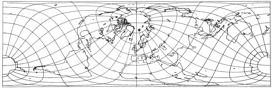
The oblique Cylindrical Equal-Area projection has been proposed with particular parameters for maps of Eurasia and Africa (Thornthwaite, 1927) and of air routes of the British Commonwealth (Poole, 1934). Different parameters are used for fig. 17. The ellipsoidal form of the oblique and transverse aspects has apparently been developed only recently (Snyder, 1985b).
FEATURES #
Like other regular cylindricals, the graticule of the normal Cylindrical Equal-Area projection consists of straight equally spaced vertical meridians perpendicular to straight unequally spaced horizontal parallels. To achieve equality of area, the parallels are spaced from the Equator in proportion to the sine of the latitude. This is the simplest equal-area projection.
The normal Cylindrical Equal-Area for the sphere is a true perspective projection onto a cylinder tangent at the Equator: The meridians are projected from the center of the sphere, and the parallels are projected with lines parallel to the equatorial plane, or orthographically from infinity. Modifications such as Behrmann’s, described above, are perspective projections onto a secant cylinder. For oblique and transverse aspects, the projection may be perspectively cast on a cylinder tangent or secant at an oblique angle, or centered on a meridian.
There is no distortion of area anywhere on the projections, and no distortion of scale and shape at the standard parallels of the normal aspect, or at the standard lines of the oblique or transverse aspects. There is extreme shape and scale distortion 90° from the central line, or at the poles on the normal aspect. These are the points which have infinite area and linear scale on the various aspects of the Mercator projection. This distortion, even on the modifications described above, is so great that there has been little use of any of the forms for world maps by professional cartographers, and many of them have strongly criticized the intensive promotion in the noncartographic community which has accompanied the presentation of one of the recent modifications.
The meridians and parallels of the transverse and oblique aspects which are straight or curved on the Mercator projection are straight or curved, respectively, on the Cylindrical Equal-Area, except that the curves are differently shaped.
In spite of the shape distortion in some portions of a world map, the projection is well suited for equal-area mapping of regions which are predominantly north-south in extent, or which have an oblique central line, or which lie near the Equator. This is true in the same sense that for mid-latitude regions which extend predominantly east-west, the Albers Equal-Area Conic projection is recommended for equal-area mapping. Actually, the normal Cylindrical Equal-Area is the limiting form of the Albers when the Equator or two parallels symmetrical about the Equator are made standard. If such regions to be mapped are smaller than the United States, the ellipsoidal form should be considered. FIGURE 14.— Lambert Cylindrical Equal-Area projection. Standard parallel is Equator. Seldom used in this form but suitable for equal-area strips near the Equator. FIGURE 15.— Bhermann Cylindrical Equal-Area projection, with standard parallels at latitude 30° N and S. Same as figure 14, but compressed east to west and expanded north to south FIGURE 16.— Transverse Cylindrical Equal-Area Projection. The central meridian long. 90°W as well as long. 90°E, coincides with the Equator of the base projection. FIGURE 17.— Oblique Cylindrical Equal-Area projection, with central oblique great circle inclined 60° to the Earth’s Equator. No distortion along this central line.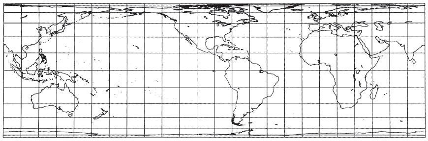
FORMULAS FOR THE SPHERE #
The geometric construction of the Cylindrical Equal-Area projection has been described above. The forward formulas for the normal aspect are as follows, given $R, \phi_s,\lambda_0,\phi$ and $\lambda$ to find $x$ and $y$ (see numerical examples):
For the oblique aspect, the alternatives used for the Oblique Mercator projection are used here, with modification only in the formulas for the $y$ coordinates:
Given two points to lie upon the central line, with latitudes and longitudes $(\phi_1, \lambda_1)$ and $(\phi_2, \lambda_2)$, and longitude increasing easterly and relative to Greenwich, the pole of the oblique transformation at $(\phi_p, \lambda_p)$ may be calculated as follows:
$$ \begin{align} \lambda_p = &\arctan[(\cos\phi_1\sin\phi_2\cos\lambda_1 - \sin\phi_1\cos\phi_2\cos\lambda_2)/ \\ &(\sin\phi_1\cos\phi_2\sin\lambda_2 - \cos\phi_1\sin\phi_2\sin\lambda_1)] \end{align} \tag{ 9-1 } $$$$ \phi_p = \arctan[-\cos(\lambda_p-\lambda_1)/\tan\phi_1] \tag{ 9-2 } $$The Fortran ATAN2 function or its equivalent should be used with equation (9-1), but not with (9-2). The other pole is located at $(-\phi_p,\lambda_p\pm\pi)$. Using the positive (northern) value of $\phi_p$, the following formulas give the rectangular coordinates for point $(\phi,\lambda)$, with $h_0$, the scale factor along the central line:$$ x= Rh_0\arctan\{[\tan\phi\cos\phi_p+\sin\phi_p\sin(\lambda-\lambda_0)]/\cos(\lambda-\lambda_0)\} \tag{ 10-4 } $$$$ y= (R/h_0)[\sin\phi_p\sin\phi-\cos\phi_p\cos\phi\sin(\lambda-\lambda_0)] \tag{ 10-5 } $$With these formulas for the oblique aspect, the origin of rectangular coordinates lies at$$ \eqalign{ \phi_0 &= 0 \cr \lambda_0 &=\phi_p + \pi/2 } \tag{ 9-6a } $$and the X axis lies along the central line, $x$ increasing easterly. The transformed poles are straight lines at $y = R$ and are as long as the central line.Given a central point $(\phi_z,\lambda_z)$ with longitude increasing easterly and relative to Greenwich, and azimuth $\gamma$ east of north of the central line through $(\phi_z,\lambda_z)$, the pole of the oblique transformation at $(\phi_p,\lambda_p)$ may be calculated as follows:
$$ \phi_p = \arcsin(\cos\phi_z\sin\gamma) \tag{ 9-7 } $$$$ \lambda_p = \arctan[-\cos\beta(-\sin\phi_z\sin\gamma)]+ \lambda_z \tag{ 9-8 } $$These values of $\phi_p$ and $\lambda_p$, may then be used in equations (10-4) and (10-5) as before.
For the inverse formulas, first for the normal aspect, given $R, \phi_s, \lambda_0, x,$ and $y$, to find $\phi$ and $\lambda$:
For the oblique aspect, equations (9-1) and (9-2) or (9-7) and (9-8) must first be used to establish the pole of the oblique transformation, if it is not known already. Then
FORMULAS FOR THE ELLIPSOID #
In the following formulas, the ellipsoid is transformed onto the authalic sphere, but the scale along the desired central line is made constant by variably compressing the scale along this central line to match that along the same path on the ellipsoid. To retain correct area, the distances perpendicular to the central line are increased by the same ratio. For the oblique aspect, the central line is not a geodesic, but is instead an oblique great circle on the authalic sphere.
For the forward formulas using the normal aspect, given $a, e, \phi_s, \lambda_0, \phi$, and $\lambda$, to find $x$ and $y$ (see numerical examples), the equations are given in the order of computation:
For the transverse aspect, the subsequent formulas for the oblique aspect may be used, but the following are simpler for the transverse alone. Given $a, e, h_0, \lambda_0, \phi_0, \phi,$ and $\lambda$, to find $x$ and $y$, first $q$ is calculated from $\phi$ using equation (3-12) above. Then
For the oblique aspect, the location of the pole $(\phi_p,\lambda_p)$ may be given, or it may be computed as described under the section on formulas for the sphere above. Points $\phi_1, \phi_2, \phi_p$ and $\phi_z$, however, are replaced in equations (9-1), (9-2), (9-7) and (9-8) with $\beta_1, \beta_2, \beta_p$ and $\beta_z$ respectively, and $\beta_p$ is finally converted to $\phi_p$, using equations (10-17) and (3-16), or just (3-18), and subscripts $p$ instead of $c$.
If the ellipsoid is either the Clarke 1866 or the International, Fourier constants may be taken from table 13. TABLE 13.— Fourier coefficients for oblique and transverse Cylindrical Equal-Area projection for the ellipsoid
For the inverse formulas for the ellipsoid, the normal aspect will be discussed first. Given $a, e, \phi_s,\lambda_0, x$, and $y$, to find $\phi$ and $\lambda$ (see p. 284 for numerical examples), $k_0$ is determined from (10-13), and
For the transverse aspect, given $a, e, h_0, \lambda_0, x$, and $y$, to find $\phi$ and $\lambda$:
For the oblique aspect, given $a, e, h_0, \phi_p, \lambda_p, x$, and $y$, to find $\phi$ and $\lambda$, Fourier coefficients are determined as described above for the forward oblique ellipsoidal formulas, while the pole location $(\phi_p,\lambda_p)$, may be determined if not provided, as described for the forward oblique spherical formulas, and $q_p$ is found from (3-12) using 90° for $\phi$. From $x, \lambda’$ is determined from an iterative inverse of (10-23):
Equation (10-24) above is used to find $F$ from $\lambda’$. Then,
For the determination of Fourier coefficients, if they are not already provided, equation (10-23) above is equivalent to the following equation which requires numerical integration:
To compute $F$ from equation (10-37) for a given $\lambda’$, first $\beta_p$ is found from $\phi_p$ using (3-12) and (3-11), subscripting $\phi$ and $\lambda$ with p. Then,
11. MILLER CYLINDRICAL PROJECTION #
SUMMARY #
- Neither equal-area nor conformal.
- Used only in spherical form.
- Cylindrical.
- Meridians and parallels are straight lines, intersecting at right angles.
- Meridians are equidistant; parallels spaced farther apart away from Equator.
- Poles shown as lines.
- Compromise between Mercator and other cylindrical projections.
- Used for world maps.
- Presented by Miller in 1942.
HISTORY AND FEATURES #
The need for a world map which avoids some of the scale exaggeration of the Mercator projection has led to some commonly used cylindrical modifications, as well as to other modifications which are not cylindrical. The earliest common cylindrical example was developed by James Gall of Edinburgh about 1855 (Gall, 1885, p. 119-123). His meridians are equally spaced, but the parallels are spaced at increasing intervals away from the Equator. The parallels of latitude are actually projected onto a cylinder wrapped about the sphere, but cutting it at lats. 45° N. and S., the point of perspective being a point on the Equator opposite the meridian being projected. It is used in several British atlases, but seldom in the United States. The Gall projection is neither conformal nor equal-area, but has a blend of various features. Unlike the Mercator, the Gall shows the poles as lines running across the top and bottom of the map.
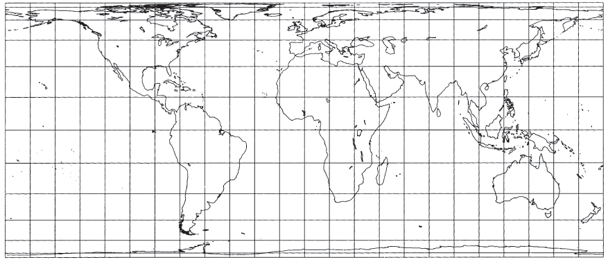
What might be called the American version of the Gall projection is the Miller Cylindrical projection (fig. 18), presented in 1942 by Osborn Maitland Miller (1897-1979) of the American Geographical Society, New York (Miller, 1942). Born in Perth, Scotland, and educated in Scotland and England, Miller came to the Society in 1922. There he developed several improved surveying and mapping techniques. An expert in aerial photography, he developed techniques for converting high-altitude photographs into maps. He led or joined several expeditions of explorers and advised leaders of others. He retired in 1968, having been best known to cartographers for several map projections, including the Bipolar Oblique Conic Conformal, the Oblated Stereographic, and especially his Cylindrical projection.
Miller had been asked by S. Whittemore Boggs, Geographer of the U.S. Department of State, to study further alternatives to the Mercator, the Gall, and other cylindrical world maps. In his presentation, Miller listed four proposals, but the one he preferred, and the one used, is a fairly simple mathematical modification of the Mercator projection. Like the Gall, it shows visible straight lines for the poles, increasingly spaced parallels away from the Equator, equidistant meridians, and is not equal-area, equidistant along meridians, nor conformal. While the standard parallels, or lines true to scale and free of distortion, on the Gall are at lats. 45° N. and S., on the Miller only the Equator is standard. Unlike the Gall, the Miller is not a perspective projection.
The Miller Cylindrical projection is used for world maps and in several atlases, including the National Atlas of the United States (USGS, 1970, p. 330-331). As Miller (1942) stated,
the practical problem considered here is to find a system of spacing the parallels of latitude such that an acceptable balance is reached between shape and area distortion. By an “acceptable” balance is meant one which to the uncritical eye does not obviously depart from the familiar shapes of the land areas as depicted by the Mercator projection but which reduces areal distortion as far as possible under these conditions * * *. After some experimenting, the [Modified Mercator (b)] was judged to be the most suitable for Mr. Boggs’s purpose * * *.
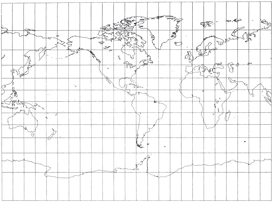
FIGURE 18.— The Miller Cylindrical Projection. A projection resembling the Mercator, but having less relative distortion in polar regions. Neither conformal nor equal-area.
FORMULAS FOR THE SPHERE #
Miller’s spacings of parallels from the Equator are the same as if the Mercator spacings were calculated for 0.8 times the respective latitudes, with the result divided by 0.8. As a result, the spacing of parallels near the Equator is very close to the Mercator arrangement.
The forward formulas, then, are as follows (see numerical example):
The inverse equations are easily derived from equations (11-1) through (11-2a):
Rectangular coordinates are given in table 14. There is no basis for an ellipsoidal equivalent, since the projection is used for maps of the entire Earth and not for local areas at large scale. TABLE 14.— Miller Cylindrical projection: Rectangular coordinates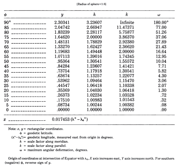
12. EQUIDISTANT CYLINDRICAL PROJECTION #
SUMMARY #
- Cylindrical.
- Neither equal-area nor conformal.
- Meridians and parallels are equidistant straight lines, intersecting at right angles.
- Poles shown as lines.
- Used for world or regional maps.
- Very simple construction.
- Used only in spherical form.
- Presented by Eratosthenes (B.C.) or Marinus (A.D. 100).
HISTORY AND FEATURES #
While the Equidistant Cylindrical projection has received limited use by the USGS and generally has limited value, it is probably the simplest of all map projections to construct and one of the oldest. The meridians and parallels are all equidistant straight parallel lines, the two sets crossing at right angles.
The projection originated probably with Eratosthenes (275?-195? B.C.), the scientist and geographer noted for his fairly accurate measure of the size of the Earth. Claudius Ptolemy credited Marinus of Tyre with the invention about A.D. 100 stating that, while Marinus had previously evaluated existing projections, the latter had chosen “a manner of representing the distances which gives the worst results of all.” Only the parallel of Rhodes (lat. 36°N.) was made true to scale on the world map, which meant that the meridians were spaced at about four-fifths of the spacing of the parallels for the same degree interval (Keuning, 1955, p. 13).
Ptolemy approved the use of the projection for maps of smaller areas, however, with spacing of meridians to provide correct scale along the central parallel. All the Greek manuscript maps for the Geographia, dating from the 13th century, use the Ptolemy modification. It was used for some maps until the 18th century, but is now used primarily for a few maps on which distortion is considered less important than the ease of displaying special information. The projection is given a variety of names such as Equidistant Cylindrical, Rectangular, La Carte Parallelogrammatique, Die Rechteckige Plattkarte, and Equirectangular (Steers, 1970, p. 135-136). It was called the projection of Marinus by Nordenskiold (1889).
If the Equator is made the standard parallel, true to scale and free of distortion, the meridians are spaced at the same distances as the parallels, and the graticule appears square. This form is often called the Plate Carrée or the Simple Cylindrical projection.
The USGS uses the Equidistant Cylindrical projection for index maps of the conterminous United states, with insets of Alaska, Hawaii, and various islands on the same projection. One is entitled “Topographic Mapping Status and Progress of Operations (7½- and 15-minute series),” at an approximate scale of 1:5,000,000. Another shows the status of intermediate-scale quadrangle mapping. Neither the scale nor the projection is marked, to avoid implying that the maps are suitable for normal geographic information. Meridian spacing is about four-fifths of the spacing of parallels, by coincidence the same as that chosen by Marinus. The Alaska inset is shown at about half the scale and with a change in spacing ratios. Individual States are shown by the USGS on other index maps using the same projection and spacing ratio to indicate the status of aerial photography.
The projection was chosen largely for ease in computerized plotting. While the boundaries on the base map may be as difficult to plot on this projection as on the others, the base map needs to be prepared only once. Overlays of digital information, which may then be printed in straight lines, may be easily updated without the use of cartographic and photographic skills. The 4:5 spacing ratio is a convenience based on computer line and character spacing and is not an attempt to achieve a particular standard parallel, which happens to fall near lat. 37° N.
FORMULAS FOR THE SPHERE #
The formulas for rectangular coordinates are almost as simple to use as the geometric construction. Given $R, \lambda_0, \phi_1, \lambda$, and $\phi$ for the forward solution, $x$ and $y$ are found thus:
13. CASSINI PROJECTION #
SUMMARY #
- Cylindrical.
- Neither equal-area nor conformal.
- Central meridian, each meridian 90" from central meridian, and Equator are straight lines.
- Other meridians and parallels are complex curves.
- Scale is true along central meridian, and along lines perpendicular to central
- meridian. Scale is constant but not true along lines parallel to central meridian on spherical form, nearly so for ellipsoid.
- Used for topographic mapping formerly in England and currently in a few other countries.
- Devised by C. F. Cassini de Thury in 1745 for the survey of France.
HISTORY #
Although the Cassini projection has been largely replaced by the Transverse Mercator, it is still in limited use outside the United States and was one of the major topographic mapping projections until the early 20th century. It was first developed by César François Cassini de Thury (1714-1784), grandson of Jean Dominique Cassini. The latter was an outstanding Italian-born astronomer who changed his given names from Giovanni Domenico after being hired in 1669 for astronomical research in Paris, and soon thereafter to begin the survey of France. Cassini de Thury was the third of four generations involved in this project, the first detailed survey of a nation. In 1745 he devised the projection which, with some modifications, still bears the family name and was used for official topographic maps of France until its replacement by the Bonne projection in 1803.
Instead of showing meridians and parallels (except for the central meridian), Cassini employed a system of squares with rectangular grid coordinates, the meridian through Paris serving as one axis. The scale along this central meridian was made correct according to the surveyed distance, thus approximately correcting for the ellipsoid (Craig, 1882, p. 80; Reignier, 1957, p. 98-99). Mathematical analysis by J. G. von Soldner in the early 19th century led to more accurate ellipsoidal formulas, and the name Cassini-Soldner is often used for the form used in topographic mapping.
FEATURES #
The spherical form of the Cassini projection (fig. 19) bears the same relation to the Equidistant Cylindrical or Plate Carrée projection that the spherical Transverse Mercator bears to the regular Mercator. Instead of having the straight meridians and parallels of the Equidistant Cylindrical, the Cassini has complex curves for each, except for the Equator, the central meridian, and each meridian 90° away from the central meridian, all of which are straight. FIGURE 19.— Cassini projection. A transverse Equidistant Cylindrical projection used for large-scale mapping in France, England, and several other countries. Largely replaced by conformal mapping.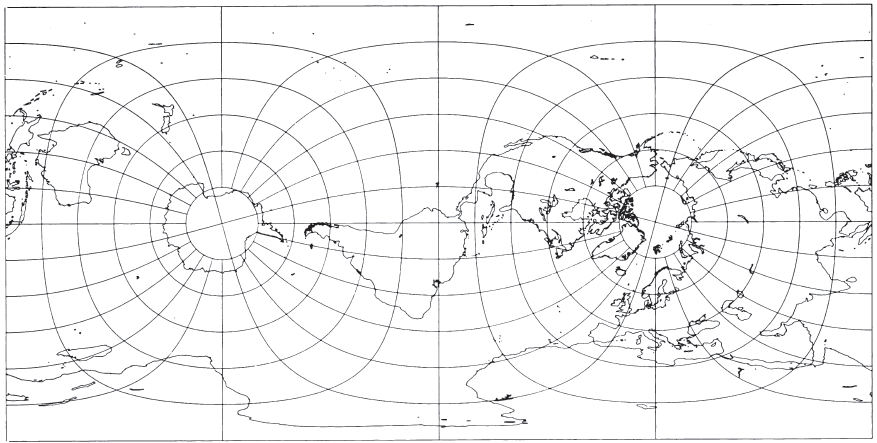
By making a given point (such as Washington, D.C.) the pole on an oblique Equidistant Cylindrical projection, the bearing and distance from that point to any other on the Earth can be read directly as two rectangular coordinates (Botley, 1951). This provides the same information as the oblique Azimuthal Equidistant projection centered on the same point. The oblique cylindrical has the advantage of offering rectangular instead of polar coordinates, but the map is much more distorted near the chosen point.
The scale is correct along the central meridian and also along any straight line perpendicular to the central meridian. It gradually increases in a direction parallel to the central meridian, as the distance from that meridian increases, but the scale is constant along any straight line on the map which is parallel to the central meridian. Therefore, the Cassini is more suitable for regions predominantly north-south in extent, such as Great Britain, than for regions extending in other directions. In this respect, it is also like the Transverse Mercator. The projection is neither equal-area nor conformal, but it has a compromise of both features.
The ellipsoidal form is computed from series which are essentially modifications of those for the ellipsoidal form of the Transverse Mercator and are suitable within only a few degrees to either side of the central meridian. The scale characteristics described above for the spherical form apply to the ellipsoidal form, except that the lines of constant scale paralleling the central meridian are not quite straight.
USAGE #
There has been little usage of the spherical version of the Cassini, but the ellipsoidal Cassini-Soldner version was adopted by the Ordnance Survey for the official survey of Great Britain during the second half of the 19th century (Steers, 1970, p. 229). Many of these maps were prepared at a scale of 1:2,600. The Cassini-Soldner was also used for the detailed mapping of many German states during the same period.
Beginning about 1920, the Ordnance Survey began to change to the Transverse Mercator because of the difficulty of measuring scale and direction on the Cassini. Nevertheless, there are several maps still in print which are based on the older projection in Great Britain, and the projection is used in a few other countries such as Cyprus, Czechoslovakia, Denmark, the Federal Republic of Germany, and Malaysia (Clifford J. Mugnier, personal comm., 1985).
A system equivalent to an oblique Equidistant Cylindrical or oblique Cassini projection was used in early coordinate transformations for ERTS (now Landsat) satellite imagery, but it was changed in 1978 to the Hotine Oblique Mercator, and in 1982 to the Space Oblique Mercator projection.
FORMULAS FOR THE SPHERE #
For the forward formulas, given $R, \phi_o, \lambda_0, \phi$, and $\lambda$, to find $x$ and $y$:
The inverse formulas for $(\phi,\lambda)$ in terms of $(x, y)$:
FORMULAS FOR THE ELLIPSOID #
For the ellipsoidal form, a set of series approximations is given for use in a zone extending 3° to 4° of longitude from the central meridian. Coordinate axes are the same as they are for the spherical formulas above. The formulas below are adapted from those provided by Clifford J. Mugnier (pers. commun., 1979; see also Clark and Clendinning, 1944).
$M_0 = M$ calculated for $\phi_0$, the latitude crossing the central meridian $\lambda_0$ at the origin of the $x, y$ coordinates. The choice of $\phi_0$ does not affect the shape of the projection.
$s =$ the scale factor at an azimuth $Az$ east of north for a given $\phi$ and $x$.
From $\phi_1$, other terms below are calculated for use in equations (13-10) and (13-11). (If $\phi_1=\pm\pi/2, \thinspace \phi=\pm90^\circ$, taking the sign of $y$, while $\lambda$ is indeterminate, and may be called $\lambda_0$.)
Hotine uses positive west longitude, x corresponding to u here, and y corresponding to -v here. Thomas uses positive west longitude, y corresponding to u here, and x corresponding to -v here. In calculations of Alaska zone 1, west longitude is positive, but u and v agree with u and v, respectively, here. ↩︎