14. ALBERS EQUAL-AREA CONIC PROJECTION #
SUMMARY #
- Conic.
- Equal-Area.
- Parallels are unequally spaced arcs of concentric circles, more closely spaced at the north and south edges of the map.
- Meridians are equally spaced radii of the same circles, cutting parallels at right angles.
- There is no distortion in scale or shape along two standard parallels, normally, or along just one.
- Poles are arcs of circles.
- Used for equal-area maps of regions with predominant east-west expanse, especially the conterminous United States.
- Presented by Albers in 1805.
HISTORY #
One of the most commonly used projections for maps of the conterminous United States is the equal-area form of the conic projection, using two standard parallels. This projection was first presented by Heinrich Christian Albers (1773-1833), a native of Luneburg, Germany, in a German periodical of 1805 (Albers, 1805; Bonacker and Anliker, 1930). The Albers projection was used for a German map of Europe in 1817, but it was promoted for maps of the United States in the early part of the 20th century by Oscar S. Adams of the Coast and Geodetic Survey as “an equal-area representation that is as good as any other and in many respects superior to all others” (Adams, 1927, p. 1).
FEATURES AND USAGE #
The Albers is the projection exclusively used by the USGS for sectional maps of all 50 States of the United States in the National Atlas of 1970, and for other U.S. maps at scales of 1:2,500,000 and smaller. The latter maps include the base maps of the United States issued in 1961, 1967, and 1972, the Tectonic Map of the United States (1962), and the Geologic Map of the United States (1974), all at 1:2,500,000. The USGS has also prepared a U.S. base map at 1:3,168,000 (1 inch = 50 miles).
Like other normal conics, the Albers Equal-Area Conic projection (fig. 20) has concentric arcs of circles for parallels and equally spaced radii as meridians. The parallels are not equally spaced, but they are farthest apart in the latitudes between the standard parallels and closer together to the north and south. The pole is not the center of the circles, but is normally an arc itself.
FIGURE 20.— Albers Equal-Area Conic projection, with standard parallels 20° and 60° N. This illustration includes all of North America to show the change in spacing of the parallels. When used for maps of the 48 conterminous States standard parallels are 29.5° and 45.5° N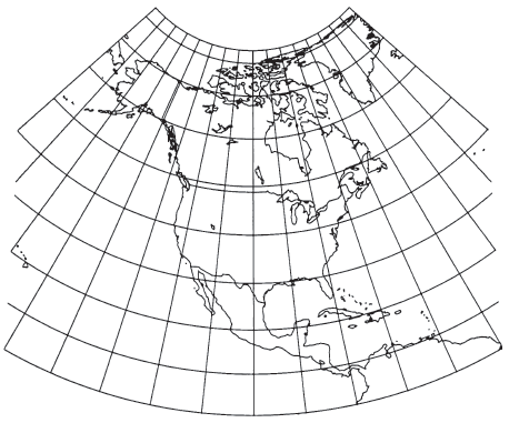
If the pole is taken as one of the two standard parallels, the Albers formulas reduce to a limiting form of the projection called Lambert’s Equal-Area Conic (not discussed here, and not to be confused with his Conformal Conic, to be discussed later). If the pole is the only standard parallel, the Albers formulas simplify to provide the polar aspect of the Lambert Azimuthal Equal-Area (discussed later). In both of these limiting cases, the pole is a point. If the Equator is the one standard parallel, the projection becomes Lambert’s Cylindrical Equal-Area (discussed earlier), but the formulas must be modified. None of these extreme cases applies to the normal use of the Albers, with standard parallels in the temperate zones, such as usage for the United States.
Scale along the parallels is too small between the standard parallels and too large beyond them. The scale along the meridians is just the opposite, and in fact the scale factor along meridians is the reciprocal of the scale factor along parallels, to maintain equal area. An important characteristic of all normal conic projections is that scale is constant along any given parallel.
To map a given region, standard parallels should be selected to minimize variations in scale. Not only are standard parallels correct in scale along the parallel; they are correct in every direction. Thus, there is no angular distortion, and conformality exists along these standard parallels, even on an equal-area projection. They may be on opposite sides of, but not equidistant from, the Equator. Deetz and Adams (1934, p. 79, 91) recommended in general that standard parallels be placed one-sixth of the displayed length of the central meridian from the northern and southern limits of the map. Hinks (1912, p. 87) suggested one-seventh instead of one-sixth. Others have suggested selecting standard parallels of conics so that the maximum scale error (1 minus the scale factor) in the region between them is equal and opposite in sign to the error at the upper and lower parallels, or so that the scale factor at the middle parallel is the reciprocal of that at the limiting parallels. Tsinger in 1916 and Kavrayskiy in 1934 chose standard parallels so that least-square errors in linear scale were minimal for the actual land or country being displayed on the map. This involved weighting each latitude in accordance with the land it contains (Maling, 1960, p. 263-266).
The standard parallels chosen by Adams for Albers maps of the conterminous United States are lats. 29.5° and 45.5°N. These parallels provide “for a scale error slightly less than 1 per cent in the center of the map, wit.h a maximum of 1¼ per cent along the northern and southern borders” (Deetz and Adams, 1934, p. 91). For maps of Alaska, the chosen standard parallels are lats. 55° and 65°N., and for Hawaii, lats. 8° and 18°N. In the latter case, both parallels are south of the islands, but they were chosen to include maps of the more southerly Canal Zone and especially the Philippine Islands. These parallels apply to all maps prepared by the USGS on the Albers projection, originally using Adams’s published tables of coordinates for the Clarke 1866 ellipsoid (Adams, 1927).
Without measuring the spacing of parallels along a meridian, it is almost impossible to distinguish an unlabeled Albers map of the United States from other conic forms. It is only when the projection is extended considerably north and south, well beyond the standard parallels, that the difference is apparent without scaling.
Since meridians intersect parallels at right angles, it may at first seem that there is no angular distortion. However, scale variations along the meridians cause some angular distortion for any angle other than that between the meridian and parallel, except at the standard parallels.
FORMULAS FOR THE SPHERE #
The Albers Equal-Area Conic projection may be constructed with only one standard parallel, but it is nearly always used with two. The forward formulas for the sphere are as follows, to obtain rectangular or polar coordinates, given $R, \phi_1, \phi_2, \phi_0, \lambda_0, \phi$, and $\lambda$ (see numerical examples):
The Y axis lies along the central meridian $\lambda_0$, $y$ increasing northerly. The X axis intersects perpendicularly at $\phi_0$, $x$ increasing easterly. If $(\lambda - \lambda_0)$ exceeds the range $\pm180°$, 360° should be added or subtracted to place it within the range. Constants $n, C$, and $\rho_0$ apply to the entire map, and thus need to be calculated only once. If only one standard parallel 4, is desired (or if $\phi_1=\phi_2$), $n=\sin\phi_1$. By contrast, a geometrically secant cone requires a cone constant $n$ of $\sin[(\phi_1+\phi_2)/2]$, slightly but distinctly different from equation (14-6). If the projection is designed primarily for the Northern Hemisphere, $n$ and $\rho$ are positive. For the Southern Hemisphere, they are negative. The scale along the meridians, using equation (4-4),
For the inverse formulas for the sphere, given $R, \phi_1, \phi_2, \phi_0, \lambda_0, x$, and $y$: $n, C$ and $\rho$, are calculated from equations (14-6), (14-5), and (14-3a), respectively. Then,
FORMULAS FOR THE ELLIPSOID #
The formulas displayed by Adams and most other writers describing the ellipsoidal form include series, but the equations may be expressed in closed forms which are suitable for programming, and involve no numerical integration or iteration in the forward form. Nearly all published maps of the United States based on the Albers use the ellipsoidal form because of the use of tables for the original base maps. (Adams, 1927, p. 1-7; Deetz and Adams, 1934, p. 93-99; Snyder, 1979a, p. 71). Given $a, e, \phi_1, \phi_2, \phi_0, \lambda_0, \phi$, and $\lambda$ (see numerical examples):
For the inverse formulas for the ellipsoid, given $a, e, \phi_1, \phi_2. \phi_0, \lambda_0, x$, and $y$: $n, C$, and $\rho_0$ are calculated from equations (14-14), (14-13), and (14-12a); respectively. Then,
Instead of the iteration, a series may be used for the inverse ellipsoidal formulas:
Polar coordinates for the Albers Equal-Area Conic are given for both the spherical and ellipsoidal forms, using standard parallels of lat. 29.5° and 45.5° N. (table 15). A graticule extended to the North Pole is shown in figure 20. TABLE 15.—Albers Equal-Area Conic projection: Polar coordinates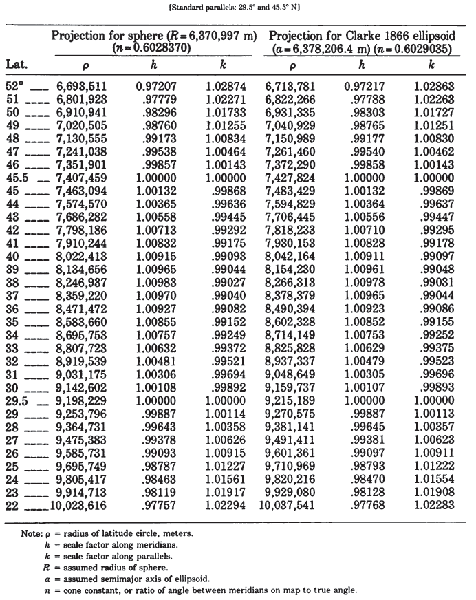
To convert coordinates measured on an existing map, the user may choose any meridian for $\lambda_0$. and therefore for the Y axis, and any latitude for $\phi_0$. The X axis then is placed perpendicular to the Y axis at $\phi_0$.