15. LAMBERT CONFORMAL CONIC PROJECTION #
SUMMARY #
- Conic
- Conformal
- Parallels are unequally spaced arcs of concentric circles, more closely spaced near the center of the map. Meridians are equally spaced radii of the same circles, thereby cutting parallels at right angles.
- Scale is true along two standard parallels, normally, or along just one.
- Pole in same hemisphere as standard parallels is a point; other pole is at infinity.
- Used for maps of countries and regions with predominant east-west expanse.
- Presented by Lambert in 1772.
HISTORY #
The Lambert Conformal Conic projection (fig. 21) was almost completely overlooked between its introduction and its revival by the U.S. Coast and Geodetic Survey (Deetz, 1918b), although France had introduced an approximate version, calling it “Lambert,” for battle maps of the First World War (Mugnier, 1983). It was the first new projection which Johann Heinrich Lambert presented in his Beitrage (Lambert, 1772), the publication which contained his Transverse Mercator described previously. In some atlases, particularly British, the Lambert Conformal Conic is called the “Conical Orthomorphic” projection.
FIGURE 21.—Lambert Conformal Conic projection, with standard parallels 20° and 60° N. North America is illustrated here to show the change in spacing of the parallels. When used for maps of the conterminous United States or individual States, standard parallels are 33° and 45° N.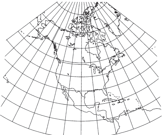
Lambert developed the regular Conformal Conic as the oblique aspect of a family containing the previously known polar Stereographic and regular Mercator projections. As he stated,
Stereographic representations of the spherical surface, as well as Mercator’s nautical charts, have the peculiarity that all angles maintain the sizes that they have on the surface of the globe. This yields the greatest similarity that any plane figure can have with one drawn on the surface of a sphere. The question has not been asked whether this property occurs only in the two methods of representation mentioned or whether these two representations, so different in appearances, can be made to approach each other through intermediate stages. * * * if there are stages intermediate to these two representations, they must be sought by allowing the angle of intersection of the meridians to be arbitrarily larger or smaller than its value on the surface of the sphere. This is the way in which I shall now proceed (Lambert, 1772, p. 28, translation by Tobler).
Lambert then developed the mathematics for both the spherical and ellipsoidal forms for two standard parallels and included a small map of Europe as an example (Lambert, 1772, p. 28-38, 87-89).
FEATURES #
Many of the comments concerning the appearance of the Albers and the selection of its standard parallels apply to the Lambert Conformal Conic when an area the size of the conterminous United States or smaller is considered. As stated before, the spacing of the parallels must be measured to distinguish among the various conic projections for such an area. If the projection is extended toward either pole and the Equator, as on a map of North America, the differences become more obvious. Although meridians are equally spaced radii of the concentric circular arcs representing parallels of latitude, the parallels become further apart as the distance from the central parallels increases. Conformality fails at each pole, as in the case of the regular Mercator. The pole in the same hemisphere as the standard parallels is shown on the Lambert Conformal Conic as a point. The other pole is at infinity. Straight lines between points approximate great circle arcs for maps of moderate coverage, but only the Gnomonic projection rigorously has this feature and then only for the sphere.
Two parallels may be made standard or true to scale, as well as conformal. It is also possible to have just one standard parallel. Since there is no angular distortion at any parallel (except at the poles), it is possible to change the standard parallels to just one, or to another pair, just by changing the scale applied to the existing map and calculating a pair of standard parallels fitting the new scale. This is not true of the Albers, on which only the original standard parallels are free from angular distortion.
If the standard parallels are symmetrical about the Equator, the regular Mercator results (although formulas must be revised). If the only standard parallel is a pole, the polar Stereographic results.
The scale is too small between the standard parallels and too large beyond them. This applies to the scale along meridians, as well as along parallels, or in any other direction, since they are equal at any given point. Thus, in the State Plane Coordinate Systems (SPCS) for States using the Lambert, the choice of standard parallels has the effect of reducing the scale of the central parallel by an amount which cannot be expressed simply in exact form, while the scale for the central meridian of a map using the Transverse Mercator is normally reduced by a simple fraction. The scale is constant along any given parallel. While it equals the nominal scale at the standard parallels, it actually changes most slowly in a north-south direction at a parallel nearly halfway between the two standard parallels.
USAGE #
It was only a couple of decades after the Coast and Geodetic Survey began publishing tables for the Lambert Conformal Conic projection (Deetz, 1918a 1918b) that the projection was adopted officially for the SPCS for States of predominantly east-west expanse. The prototype was the North Carolina Coordinate System, established in 1933. Within a year or so, similar systems were devised for many other States, while a Transverse Mercator system was prepared for the remaining States. One or more zones is involved in the system for each State (see table 8) (Mitchell and Simmons, 1945, p. vi). In addition, the Lambert is used for the Aleutian Islands of Alaska, Long Island in New York, and northwestern Florida, although the Transverse Mercator (and Oblique Mercator in one case) is used for the rest of each of these States.
The Lambert Conformal Conic is used for the 1:1,000,000-scale regional world aeronautical charts, the 1:500,000-scale sectional aeronautical charts, and 1:500,000-scale State base maps (all 48 contiguous States1 have the same standard parallels of lat. 33° and 45° N., and thus match). Also cast on the Lambert are most of the 1:24,000-scale 7½-minute quadrangles prepared after 1957 which lie in zones for which the Lambert is the base for the SPCS. In the latter case, the standard parallels for the zone are used, rather than parameters designed for the individual quadrangles. Thus, all quadrangles for a given zone may be mosaicked exactly. (The projection used previously was the Polyconic, and some recent quadrangles are being produced to the Universal Transverse Mercator projection.)
The Lambert Conformal Conic has also been adopted as the official topographic projection for some other countries. It appears in The National Atlas (USGS, 1970, p. 116) for a map of hurricane patterns in the North Atlantic, and the Lambert is used by the USGS for a map of the United States showing all 50 States in their true relative positions. The latter map is at scales of both 1:6,000,000 and 1:10,000,000, with standard parallels 37° and 65° N.
In 1962, the projection for the International Map of the World at a scale of 1:1,000,000 was changed from a modified Polyconic to the Lambert Conformal Conic between lats. 84° N. and 80° S. The polar Stereographic projection is used in the remaining areas. The sheets are generally 6° of longitude wide by 4° of latitude high. The standard parallels are placed at one-sixth and five-sixths of the latitude spacing for each zone of 4° latitude, and the reference ellipsoid is the International (United Nations, 1963, p. 9-27). This specification has been subsequently used by the USGS in constructing several maps for the IMW series.
Perhaps the most recent new topographic use for the Lambert Conformal Conic projection by the USGS is for middle latitudes of the 1:1,000,000-scale geologic series of the Moon and for some of the maps of Mercury, Mars, and Jupiter’s satellites (see table 6).
FORMULAS FOR THE SPHERE #
For the projection as normally used, with two standard parallels, the equations for the sphere may be written as follows: given $R, \phi_1, \phi_2, \phi_0, \lambda_0, \phi$, and $\lambda$ (see numerical examples):
$\phi_1,\phi_2=$ standard parallels.
The Y axis lies along the central meridian $\lambda_0$, $y$ increasing northerly; the X axis intersects perpendicularly at $\phi_0, x$ increasing easterly. If $(\lambda-\lambda_0)$ exceeds the range $\pm180°$, 360° should be added or subtracted. Constants $n, F$, and $\rho_0$ need to be determined only once for the entire map.
If only one standard parallel is desired, equation (15-3) is indeterminate, but $n=\sin\phi_1$. The scale along meridians or parallels, using equations (4-4) or (4-5),
For the inverse formulas for the sphere, given $R,\phi_1,\phi_2,\phi_0,\lambda_0, x$ and $y$: $n, F,$ and $\rho_0$ are calculated from equations (15-3), (15-2), and (15-1a), respectively.Then,
The standard parallels normally used for maps of the conterminous United States are lats. 33° and 45° N., which give approximately the least overall error within those boundaries. The ellipsoidal form is used for such maps, based on the Clarke 1866 ellipsoid (Adams, 1918).
The standard parallels of 33° and 45° were selected by the USGS because of the existing tables by Adams (1918), but Adams chose them to provide a maximum scale error between latitudes 30.5° and 47.5° of one-half of 1 percent. A maximum scale error of 2.5 percent occurs in southernmost Florida (Deetz and Adams, 1934, p. 80). Other standard parallels would reduce the maximum scale error for the United States, but at the expense of accuracy in the center of the map.
FORMULAS FOR THE ELLIPSOID #
The ellipsoidal formulas are essential when applying the Lambert Conformal Conic to mapping at a scale of 1:100,000 or larger and important at scales of 1:5,000,000. Given $a, e, \phi_1, \phi_2, \phi_0, \lambda_0, \phi$, and $\lambda$ (see numerical examples):
When the above equations for the ellipsoidal form are used, they give values of $n$ and $\rho$ slightly different from those in the accepted tables of coordinates for a map of the United States, according to the Lambert Conformal Conic projection. The discrepancy is 35-50 m in the radius and 0.0000035 in $n$. The rectangular coordinates are correspondingly affected. The discrepancy is less significant when it is realized that the radius is measured to the pole, and that the distance from the 50th parallel to the 25th parallel on the map at full scale is only 12 m out of 2,800,000 or 0.0004 percent. For calculating convenience 60 years ago, the tables were, in effect, calculated using instead of equation (15-9),
For the existing tables, then, $\phi_g$, the geocentric latitude, was used for convenience in place of $\chi$ , the conformal latitude (Adams, 1918, p. 6-9, 34). A comparison of series equations (3-3) and (3-30), or of the corresponding columns in table 3, shows that the two auxiliary latitudes $\chi$ and $\phi_g$ are numerically very nearly the same.
There may be much smaller discrepancies found between coordinates as calculated on modern computers and those listed in tables for the SPCS. This is due to the slightly reduced (but sufficient) accuracy of the desk calculators of 30-40 years ago and the adaptation of formulas to be more easily utilized by them. To obtain SPCS coordinates, the appropriate “false easting” is added to $x$ after calculation using (14-1).
The inverse formulas for ellipsoidal coordinates, given $a, e, \phi_1, \phi_2, \phi_0, \lambda_0, x$, and $y$: $n, F$, and $\rho_0$ are calculated from equations (15-8), (15-10), (15-7a), respectively . Then
Equation (7-9) involves rapidly converging iteration: Calculate t from (15-11). Then, assuming an initial trial $\phi$ equal to $(\pi/2−2\arctan t)$ in the right side of equation (7—9) , calculate $\phi$ on the left side. Substitute the calculated $\phi$ into the right side, calculate a new $\phi$, etc., until $\phi$ does not change significantly from the preceding trial value of $\phi$.
To avoid iteration, series (3-5) may be used with (7-13) in place of (7-9).
If rectangular coordinates for maps based on tables using geocentric latitude are to be converted to latitude and longitude, the inverse formulas are the same as those above except that equation (15-9b) is used instead of (15-9) for calculations leading to $n, F$, and $\rho_0$, and equation (7-9) or (3-5) and (7-13), is replaced with the following which does not involve iteration:
Polar coordinates for the Lambert Conformal Conic are given for both the spherical and ellipsoidal forms using standard parallels of 33° and 45° N, (table 16). The data based on geocentric latitude are given for comparison. A graticule extending to the North Pole is shown in figure 21. TABLE 16.—Lambert Conformal Conic projection: Polar coordinates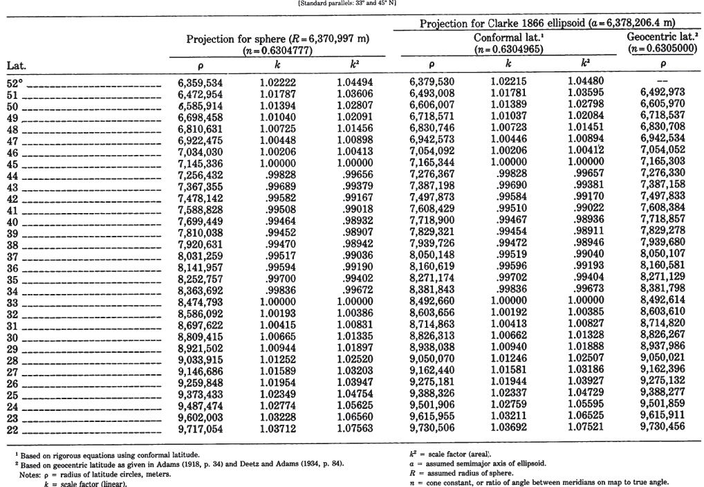
To convert from tabular rectangular coordinates to $\phi$ and $\lambda$, it is necessary to subtract any “false easting” from $x$ and “false northing” from $y$ before inserting $x$ and $y$ into the inverse formulas. To convert coordinates measured on an existing Lambert Conformal Conic map (or other regular conic projection), the user may choose any meridian for $\lambda_0$ and therefore for the Y axis , and any latitude for $\phi_0$. The X axis then is placed perpendicular to the Y axis at $\phi_0$.
For Hawaii, the standard parallels are lats. 20° 40’ and 23° 20’ N.; the corresponding base map was not prepared for Alaska. ↩︎