16. EQUIDISTANT CONIC PROJECTION #
SUMMARY #
- Conic.
- Equidistant.
- Parallels, including poles, are arcs of concentric circles, equally spaced for the sphere, at true spacing for the ellipsoid.
- Meridians are equally spaced radii of the same circles, thereby cutting parallels at right angles.
- Scale is true along all meridians and along one or two standard parallels.
- Used for maps of small countries and regions and of larger areas with predominant east-west expanse.
- Rudimentary form developed by Claudius Ptolemy about A.D. 150
HISTORY #
The simplest kind of conic projection is the Equidistant Conic, often called Simple Conic, or just Conic projection. It is the projection most likely to be found in atlases for maps of small countries, with its equally spaced straight meridians and equally spaced circular parallels. A rudimentary version was described by the astronomer and geographer Claudius Ptolemy about A.D. 150. Probably born in Greece about A.D. 90, he spent most of his life in or near Alexandria, Egypt, and died about A.D. 168. His greatest works were the Almagest, describing his scientific theories, and the Geographia, which dwelt on mapmaking. These were revived in the 15th century as the most authoritative existing standards.
In developing this projection, Ptolemy did not discuss cones, and a cone would not properly fit his specifications, but he said (Geographia, Book 1, ch. 20):
When we cast a glance upon the middle of the northern quarter of the globe in which the greatest part of the oikumene [or ecumene, or inhabited world] lies, then the meridians give the impression of being straight lines if we turn the globe thus that the meridians successively come out of their sideward situation right before the spectator, so that the eye comes in their plane. The parallels give clearly the impression of arcs of circles which turn their convex side to the south (Keuning, 1955, p. 9).
Ptolemy’s conic projection extends from latitudes approximating 63°N. to 16°S. Although meridians north of the Equator fan out as straight radii from the center of the circular parallels, they break at the Equator to connect with straight lines to points along the southernmost parallel which are the same distance apart as corresponding points at 16°N.
Johannes Ruysch (?-1533) modified this approach to continue meridians as straight radii below the Equator in a world map of 1508, and Gerardus Mercator made other modifications in the mid-16th century. The Equidistant Conic with two standard parallels is credited to Joseph Nicolas De l’Isle (1688- 1768), of an illustrious French mapmaking family. He used it for a map of Russia in 1745. There were differences in his approach, however, which resulted in meridians which are not radii of the circular arcs representing the circles.
Several Scot (Murdoch), Swiss (Euler), English (Everett), and Russian (Vitkovskiy, Kavrayskiy, and others) mathematicians published papers between 1758 and 1934 describing means of selecting the two standard parallels so that distortion is minimized using various criteria. Each of them used the same basic conic projection with concentric circular parallels and straight meridians for radii (Snyder, 1978a). The name of one of them, V. V. Kavrayskiy (or Kavraisky), has been mistakenly applied in some U.S. literature to the basic projection, but his contribution did not occur until 1934.
The Equidistant Conic projection (fig. 22) is neither conformal (like the Lambert Conformal Conic) nor equal-area (like the Albers), but it serves as a compromise between them. The Lambert parallels are more widely spaced away from the central parallel, and the Albers parallels become closer together. The parallels on the Equidistant Conic remain equally spaced on the spherical version (as they are on the sphere) and nearly so on the ellipsoidal version (with the same spacing as the distances along the meridians on the ellipsoid).
As on other normal conics, the meridians are equally spaced radii of the concentric circular arcs which form the parallels. The meridians are spaced at equal angles which are less than the true angles between the meridians; the ratio is called the cone constant, as it is on other conic projections. The poles are normally also plotted as circular arcs.
Either one or two parallels may be made standard or true to scale. There is no shape, area, or scale distortion along the standard parallels. While meridians are at correct scale everywhere, the scale along the parallels between the standard parallels (if there are two) is too small, and the scale along parallels beyond the standard parallel(s) is too great.
If the one standard parallel is the Equator, the Equidistant Conic projection becomes the Plate Carrée form of the Equidistant Cylindrical, but the formulas must be changed. If the two standard parallels are symmetrical about the Equator, the Equirectangular results. If the standard parallel is the pole, the Azimuthal Equidistant projection is obtained. FIGURE 22.—Equidistant Conic projection, with standard parallels 20° and 60° N. All of North America is included to show that parallels remain equidistant. Compare figures 20 and 21.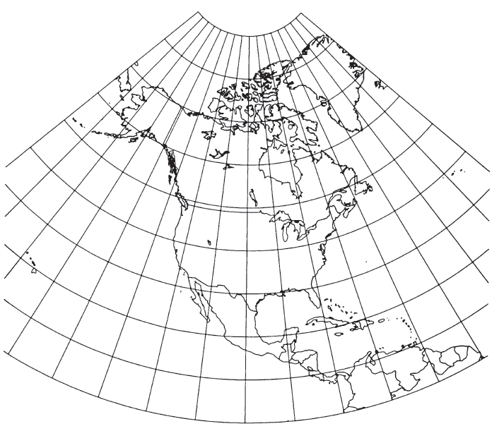
USAGE #
The Equidistant Conic projection is commonly used in the spherical form in atlases for maps of small countries. Its only use by the USGS has been in an approximate ellipsoidal form for Alaska Maps “B” and “E,” but the projection name applied is “Modified Transverse Mercator” (see p. 63), due to the original manner of construction. The formulas for the ellipsoidal version were apparently first published in Snyder (1978a), although there may be several de facto usages of the ellipsoidal form such as the above. For example, the New Mexico Planning Survey in effect devised such a projection in 1936 for the mapping of that State, calling it a “Modified Conic Projection” (Thomas E. Henderson, pers. comm., 1985).
FORMULAS FOR THE SPHERE #
For the Equidistant Conic projection with two standard parallels, given $R, \phi1, \phi2, \phi_0, \lambda_0, \phi,$ and $\lambda$, to find $x$ and $y$ (see numerical examples):
$\phi_0, \lambda_0 =$ the latitude and longitude, for the origin of the rectangular coordinates.
$\phi_1,\phi_2=$ standard parallels.
The Y axis lies along the central meridian $\lambda_0$, $y$ increasing northerly. The X axis intersects perpendicularly at $\phi_0$, $x$ increasing easterly. If $(\lambda - \lambda_0)$ exceeds the range $\pm180°$, 360° should be added or subtracted to place it within the range. Constants $n, G$, and $\rho_0$ need to be determined only once for the entire map.
If only one standard parallel $\phi_1$, is desired, equation (16-4) is indeterminate, but $n = \sin\phi_1$. The scale $h$ along meridians is 1.0. Along parallels, using equation (4-5), the scale is
The maximum angular deformation may be calculated from equation (4-9). As on other regular conics, distortion is only a function of latitude.
For the inverse formulas for the sphere, given $R, \phi1, \phi2, \phi_0, \lambda_0, x,$ and $y$ to find $\phi$ and $\lambda$: $n, G$, and $\rho_0$ are calculated from equations (16-4), (16-3), and (16-2), respectively. Then,
FORMULAS FOR THE ELLIPSOID #
For mapping of regions smaller than the United States at scales greater than 1:5,000,000, using the Equidistant Conic projection, the ellipsoidal formulas should be considered. Given $a, e, \phi_1, \phi_2, \phi_0, \lambda_0, \phi$ and $\lambda$, to find $x$ and $y$ (see numerical examples):
with the same subscripts 1,2, or none applied to $m$ and $\phi$ in equation (14-15), and 0, 1, 2, or none applied to $M$ and $\phi$ in equation (3-21). For improved computational efficiency using the series, see p. 19. As with other conics, a negative $n$ and $\rho$ result for projections centered in the Southern Hemisphere. If $\phi_1 = \phi_2$ for the Equidistant Conic with a single standard parallel, equation (16-10) is indeterminate, but $n = \sin\phi_1$. Origin and orientation of axes for x and y are the same as those for the spherical form. Constants $n, G,$ and $\rho_0$ may be determined just once for the entire map.
For the inverse formulas for the ellipsoid, given $a, e, \phi_1, \phi_2, \phi_0, \lambda_0, x,$ and $y$, to find $\phi$ and $\lambda$: $n, G,$ and $\rho_0$ are calculated from equations (16-10), (16-11), and (16-9), respectively. Then
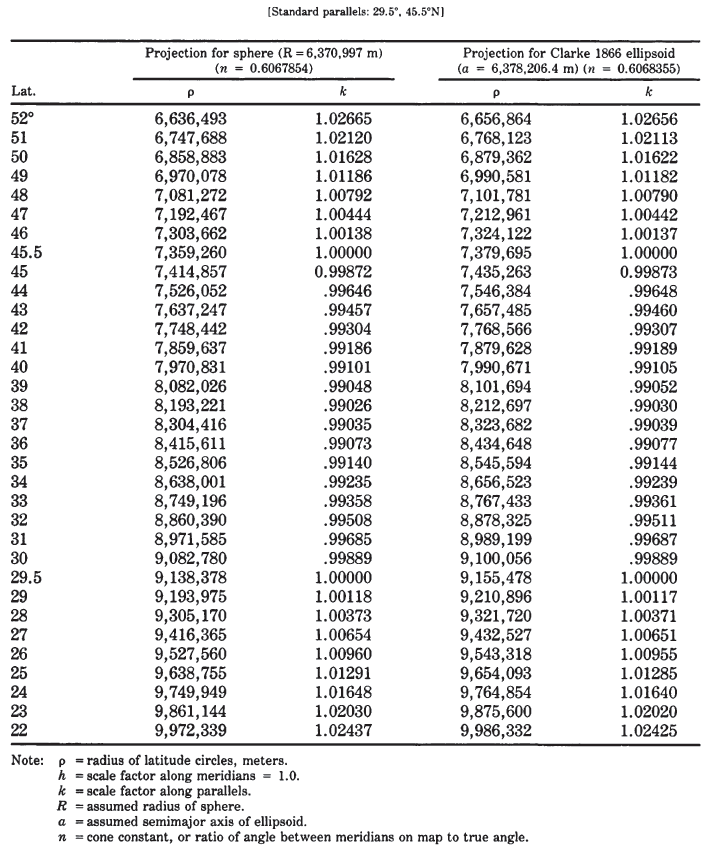
Polar coordinates for the Equidistant Conic projection for a map of the United States, assuming standard parallels of lat. 29.5° and 45.5°N., are listed in table 17 for both the spherical and ellipsoidal forms. A graticule extended to the North Pole is shown in figure 22. TABLE 17.— Equidistant Conic projection: Polar coordinates