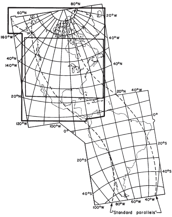
Two oblique conic projections, side-by-side, but with poles 104° apart.
Conformal.
Meridians parallels are complex curves, intersecting at right angles.
Scale is true along two standard transformed parallels on each conic projection, neither of these lines following any geographical meridian or parallel.
Very small deviation from conformality, where the two conic projections join.
Specially developed for a map of the Americas. Used only in spherical form.
A “tailor-made” projection is one designed for a certain geographical area. O. M. Miller used the term for some projections which he developed for the American Geographical Society (AGS) or for their clients. The Bipolar Oblique Conic Conformal projection, developed with William A. Briesemeister, was presented in 1941 and designed specifically for a map of North and South America constructed in several sheets by the AGS at a scale of 1:5,000,000 (Miller, 1941).
It is an adaptation of the Lambert Conformal Conic projection to minimize scale error over the two continents by accommodating the fact that North America tends to curve toward the east as one proceeds from north to south, while South America tends to curve in the opposite direction. Because of the relatively small scale of the map, the Earth was treated as a sphere. To construct the map, a great circle arc 104° long was selected to cut through Central America from southwest to
northeast, beginning at lat. 20° S. and long. 110° W. and terminating at lat. 45°N.
and the resulting longitude of about 19°59'36" W.
The former point is used as the pole and as the center of transformed parallels of latitude for an Oblique Conformal Conic projection with two standard parallels (at polar distances of 31° and 73°) for all the land in the Americas southeast of the 104° great circle arc. The latter point serves as the pole and center of parallels for an identical projection for all land northwest of the same arc. The inner and outer standard parallels of the northwest portion of the map, thus, are tangent to the outer and inner standard parallels, respectively, of the southeast portion, touching at the dividing line (104°-31° = 73°).
The scale of the map was then increased by about 3.5 percent, so that the linear scale error along the central parallels (at a polar distance of 52°, halfway between 31° and 73°) is equal and opposite in sign (-3.5 percent) to the scale error along the two standard parallels (now +3.5 percent) which are at the normal map limits. Under these conditions, transformed parallels at polar distances of about 36.34° and 66.58° are true to scale and are actually the standard transformed parallels.
The use of the Oblique Conformal Conic projection was not original with Miller and Briesemeister. The concept involves the shifting of the graticule of meridians and parallels for the regular Lambert Conformal Conic so that the pole of the projection is no longer at the pole of the Earth. This is the same principle as the transformation for the Oblique Mercator projection. The bipolar concept is unique, however, and it has apparently not been used for any other maps.
FIGURE 23.— Bipolar Oblique Conic Conformal projection used for various geologic maps. The American Geographical Society, under O. M. Miller, prepared the base map used by the USGS. (Prepared by Tau Rho Alpha.)
The Geological Survey has used the North American portion of the map for the Geologic Map (1965), the Basement Map (1967), the Geothermal Map, and the Metallogenic Map, all retaining the original scale of 1:5,000,000. The Tectonic Map of North America (1969) is generally based on the Bipolar Oblique Conic Conformal, but there are modifications near the edges. An oblique conic projection about a single transformed pole would suffice for either one of the continents alone, but the AGS map served as an available base map at an appropriate scale. In 1979, the USGS decided to replace this projection with the Transverse Mercator for a map of North America.
The projection is conformal, and each of the two conic projections has all the characteristics of the Lambert Conformal Conic projection, except for the important difference in location of the pole, and a very narrow band near the center. While meridians and parallels on the oblique projection intersect at right angles because the map is conformal, the parallels are not arcs of circles, and the meridians are not straight, except for the peripheral meridian from each transformed pole to the nearest normal pole.
The ‘scale is constant along each circular arc centered on the transformed pole for the conic projection of the particular portion of the map. Thus, the two lines at a scale factor of 1.035, that is, both pairs of the official standard transformed parallels, are mapped as circular arcs forming the letter “S.” The 104° great circle arc separating the two oblique conic projections is a straight line on the map, and all other straight lines radiating from the poles for the respective conic projections are transformed meridians and are therefore great circle routes. These straight lines are not normally shown on the finished map.
At the juncture of the two conic projections, along the 104" axis, there is actually a slight mathematical discontinuity at every point except for the two points at which the transformed parallels of polar distance 31° and 73° meet. If the conic projections are strictly followed, there is a maximum discrepancy of 1.6 mm at the 1:5,000,000 scale at the midpoint of this axis, halfway between the poles or between the intersections of the axis with the 31° and 73° transformed parallels. In other words, a meridian approaching the axis from the south is shifted up to 1.6 mm along the axis as it crosses. Along the axis, but beyond the portion between the lines of true scale, the discrepancy increases markedly, until it is over 240 mm at the transformed poles. These latter areas are beyond the needed range of the map and are not shown, just as the polar areas of the regular Lambert Conformal Conic are normally omitted. This would not happen if the Oblique Equidistant Conic projection were used.
The discontinuity was resolved by connecting the two arcs with a straight line tangent to both, a convenience which leaves the small intermediate area slightly
nonconformal. This adjustment is included in the formulas below.
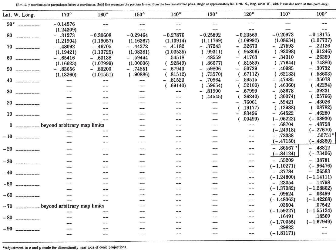
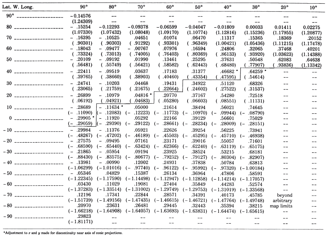
The original map was prepared by the American Geographical Society, in an era when automatic plotters and easy computation of coordinates were not yet present. Map coordinates were determined by converting the geographical coordinates of a given graticule intersection to the transformed latitude and longitude based on the poles of the projection, then to polar coordinates according to the conformal projection, and finally to rectangular coordinates relative to the selected origin.
The following formulas combine these steps in a form which may be programmed for the computer. First, various constants are calculated from the above parameters, applying to the entire map. Since only one map is involved, the numerical values are inserted in formulas, except where the numbers are transcendental and are referred to by symbols.
If the southwest pole is at point A, the northeast pole is at point B, and the center point on the axis is C,
$$ \begin{align}
\lambda_b &= -110^\circ +\arccos\{[\cos 104^\circ-\sin(-20^\circ)\sin45^\circ]/[\cos(-20^\circ)\cos45^\circ]\} \\
&= -19^\circ59'36^" \text{ long., the longitude of B (negative is west long.)}
\end{align} \tag{ 17-1 } $$
$$ \begin{align}
n &= (\ln\sin31^\circ-\ln\sin73^\circ)/[\ln\tan(31^\circ/2)-\ln\tan(73^\circ/2)] \\
&= 0.63056 \text{, the cone constant for both conic projections}
\end{align} \tag{ 17-2 } $$
$$ \begin{align}
F_0 &= R\sin31^\circ/[n\tan^n(31^\circ/2)] \\
&= 1.83376\,R \text{,where R is the radius of the globe at the scale of the map.}\\
&\ \ \text{ For the 1:5,000,000 map, R was taken as 6,371,221 m, the radius of a}\\
&\ \ \text{ sphere having a volume equal to that of the International ellipsoid.}
\end{align} \tag{ 17-3 } $$
$$ \begin{align}
k_0 &= 2/[1+n\,F_0\tan^n26^\circ/(R\sin52^\circ)] \\
&= 1.03462, \text{ the scale factor by which the coordinates are multiplied}\\
&\ \ \text{to balance the errors}
\end{align} \tag{ 17-4 } $$
$$ \begin{align}
F &= k_0F_0 \\
&= 1.89725\,R \text{ , a convenient constant}
\end{align} \tag{ 17-5 } $$
$$ \begin{align}
Az_{AB} &=&&\arccos\{[\cos(-20^\circ)\sin(45^\circ) - \sin(-20^\circ)\cos 45^\circ \\
&&&\cos(\lambda_B+110^\circ)]/\sin104^\circ\} \\
&=&&46.78203^\circ \text{ , the azimuth east of north of B from A}
\end{align} \tag{ 17-6 } $$
$$ \begin{align}
Az_{BA} &=&&\arccos\{[\cos45^\circ\sin(-20^\circ) - \sin45^\circ\cos(-20^\circ) \\
&&&\cos(\lambda_B+110^\circ)]/\sin104^\circ\} \\
&=&&46.78203^\circ \text{ , the azimuth west of north of A from B}
\end{align} \tag{ 17-7 } $$
$$ \begin{align}
T &=\tan^n(31^\circ/2)+\tan^n(73^\circ/2) \\
&= 1.27247 \text{ , a convenient constant}
\end{align} \tag{ 17-8 } $$
$$ \begin{align}
\rho_c &= 1/2F\,T \\
&= 1.20709\,R \text{ , the radius of the center point of the axis from either pole}
\end{align} \tag{ 17-9 } $$
$$ \begin{align}
z_c &= 2\arctan(T/2)^{1/n} \\
&= 52.03888^\circ \text{ , the polar distance of the center point from either pole}
\end{align} \tag{ 17-10 } $$
Note that $z_c$, would be exactly 52°, if there were no discontinuity at the axis. The values of $\phi_c, \lambda_c,$ and $Az$, are calculated as if no adjustment were made at the axis due to the discontinuity. Their use is completely arbitrary and only affects positions of the arbitrary X and Y axes, not the map itself. The adjustment is included in formulas for a given point.
$$ \begin{align}
\phi_c &= \arcsin[\sin(-20^\circ)\cos z_c + \cos(-20^\circ)\sin z_c/\cos Az_{AB}] \\
&= 17^\circ16'28^" \text {N. lat., the latitude of center point, on the} \\
& \ \ \text{ southern-cone side of the axis}
\end{align} \tag{ 17-11 } $$
$$ \begin{align}
\lambda_c &= \arcsin(\sin z_c\sin Az_{AB}/\cos\phi_c)-110^\circ \\
&= -73^\circ00'27^" \text {long., the longitude of the center point, on the}\\
& \ \ \text{southern-cone side of the axis}
\end{align} \tag{ 17-12 } $$
$$ \begin{align}
Az_c &= \arcsin[\cos(-20^\circ)\sin Az_{AB}/\cos\phi_c] \\
&= 45.81997^\circ \text{, the azimuth east of north of the axis at the center point,} \\
& \ \ \text{ relative to meridian $\lambda_c$, on the southern-cone side of the axis}
\end{align} \tag{ 17-13 } $$
The remaining equations are given in the order used, for calculating rectangular coordinates for various values of latitude $\phi$ and longitude $\lambda$ (measured east from Greenwich, or with a minus sign for the western values used here). There are some conditional transfers and adjustments which would apply only if a map extending well beyond the regions of interest were to be plotted; these are omitted to avoid unnecessary complication. It must be established first whether point $(\phi, \lambda)$ is north or south of the axis, to determine which conic projection is involved. With these formulas, it is done by comparing the azimuth of point $(\phi, \lambda)$ with the azimuth of the axis, all as viewed from B (see p. 301 for numerical examples):
$$ \begin{align}
z_B &= \arccos[\sin 45^\circ\sin\phi+\cos 45^\circ\cos\phi\cos(\lambda_B-\lambda)] \\
&= \text {polar distance of $(\phi, \lambda)$ from pole B}
\end{align} \tag{ 17-14 } $$
$$ \begin{align}
Az_B &=\arctan\{\sin(\lambda_B-\lambda)/[\cos 45^\circ\tan\phi - \sin 45^\circ\cos(\lambda_B-\lambda)]\} \\
&= \text{azimuth of $(\phi, \lambda)$ west of north, viewed from B}
\end{align} \tag{ 17-15 } $$
If $Az_B$, is greater than $Az_{BA}$ (from equation
(17-7)), go to equation
(17-23). Otherwise proceed to equation (17-16) for the projection from pole $B$.
$$ \rho_B = F\tan^{n}½z_B \tag{ 17-16 } $$
$$ \begin{align}
k &=\rho_Bn/(R\sin z_B) \\
&= \text{ scale factor at point $(\phi,\lambda)$, disregarding small adjustment near axis}
\end{align} \tag{ 17-17 } $$
using constants from equations
(17-2),
(17-3),
(17-7), and
(17-9) for rectangular coordinates relative to the axis. To change to non-skewed rectangular coordinates, go to equations
(17-32) and
(17-33). The following formulas give coordinates for the projection from pole $A$.
$$ \begin{align}
z_A &= \arccos[\sin(-20^\circ)\sin\phi + \cos(-20^\circ) \cos\phi\cos(\lambda+110^\circ)] \\
&= \text {polar distance of $(\phi, \lambda)$ from pole $A$}
\end{align} \tag{ 17-23 } $$
$$ \begin{align}
Az_A &= \arctan\{ \sin(\lambda+110^\circ)/[\cos(-20^\circ)\tan\phi-\sin(-20^\circ)\cos(\lambda+110^\circ)]\} \\
&= \text{azimuth of $(\phi, \lambda)$ east of north, viewed from $A$}
\end{align} \tag{ 17-24 } $$
$$ \rho_A = F\tan^{n/2}z_A \tag{ 17-25 } $$
$$
k =\rho_An/(R\sin z_A) = \text{ scale factor at point $(\phi,\lambda)$}
\tag{ 17-26 } $$
$$ x = -x'\cos{Az_c} - y'\sin{Az_c} \tag{ 17-32 } $$
$$ y = -y'\cos{Az_c} + x'\sin{Az_c} \tag{ 17-33 } $$
where the center point at $(\phi_c, \lambda_c)$ is approximately the origin of $(x, y)$ coordinates, the Y axis increasing due north and the X axis due east from the origin. (The meridian and parallel actually crossing the origin are shifted by about $3’$ of arc, due to the adjustment at the axis, but their actual values do not affect the calculations here.)
For the inverse formulas for the Bipolar Oblique Conic Conformal, the constants for the map must first be calculated from equations
(17-1)-
(17-13). Given x and y coordinates based on the above axes, they are then converted to the skew coordinates:
and use this value to recalculate equations (17-39), (17-40), and (17-41), repeating until $\rho_B$, found in (17-41) changes by less than a predetermined convergence.
Then,
and use this value to recalculate equations (17-48), (17-49), and (17-50), repeating until $\rho_A$, found in equation (17-50) changes by less than a predetermined
convergence. Then,