18. POLYCONIC PROJECTION #

SUMMARY #

Neither conformal nor equal-area.
Parallels of latitude (except for Equator) are arcs of circles, but are not concentric.
Central meridian and Equator are straight lines; all other meridians are complex curves.
Scale is true along each parallel and along the central meridian, but no parallel is “standard.”
Free of distortion only along the central meridian.
Used almost exclusively in slightly modified form for large-scale mapping in the United States until the 1950’s.
Was apparently originated about 1820 by Hassler.

HISTORY #

Shortly before 1820, Ferdinand Rudolph Hassler (fig. 24) began to promote the Polyconic projection, which was to become a standard for much of the official mapping of the United States (Deetz and Adams, 1934, p. 58-60).

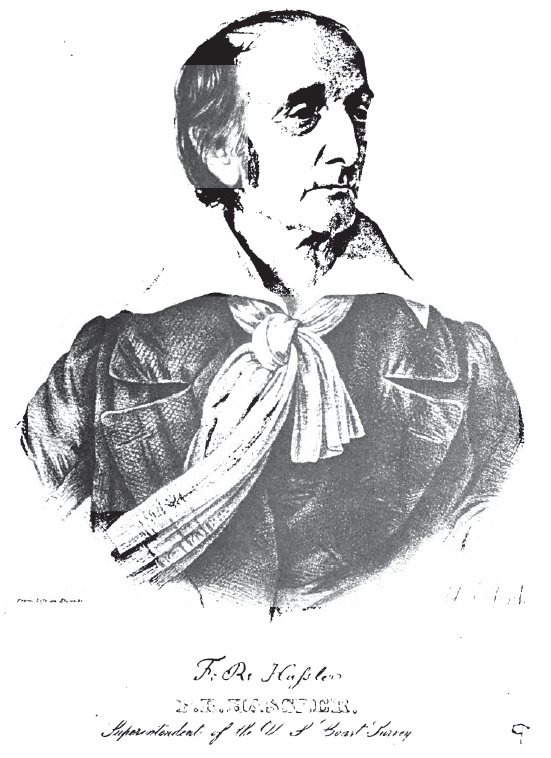
Born in Switzerland in 1770, Hassler arrived in the United States in 1805 and was hired 2 years later as the first head of the Survey of the Coast. He was forced to wait until 1811 for funds and equipment, meanwhile teaching to maintain income. After funds were granted, he spent 4 years in Europe securing equipment. Surveying began in 1816, but Congress, dissatisfied with the progress, took the Survey from his control in 1818. The work only foundered. It was returned to Hassler, now superintendent, in 1832. Hassler died in Philadelphia in 1843 as a result of exposure after a fall, trying to save his instruments in a severe wind and hailstorm, but he had firmly established what later became the U.S. Coast and Geodetic Survey (Wraight and Roberts, 1957) and is now the National Ocean Service.

The Polyconic projection, usually called the American Polyconic in Europe, achieved its name because the curvature of the circular arc for each parallel on the map is the same as it would be following the unrolling of a cone which had been wrapped around the globe tangent to the particular parallel of latitude, with the parallel traced onto the cone. Thus, there are many (“poly-”) cones involved, rather than the single cone of each regular conic projection. As Hassler himself described the principles, “[t]his distribution of the projection, in an assemblage of sections of surfaces of successive cones, tangents to or cutting a regular succession of parallels, and upon regularly changing central meridians, appeared to me the only one applicable to the coast of the United States” (Hassler, 1825, p. 407-408).

The term “polyconic” is also applied generically by some writers to other projections on which parallels are shown as circular arcs. Most commonly, the term applies to the specific projection described here.

**FIGURE 25**.— North America on a Polyconic projection grid, central meridian long. 100° W., using a 10° interval. The parallels are arcs of circles which are not concentric, but have radii equal to the radius of curvature of the parallel at the Earth’s surface. The meridians are complex curves formed by connecting points marked off along the parallels at their true distances. Used by the USGS for topographic quadrangle maps.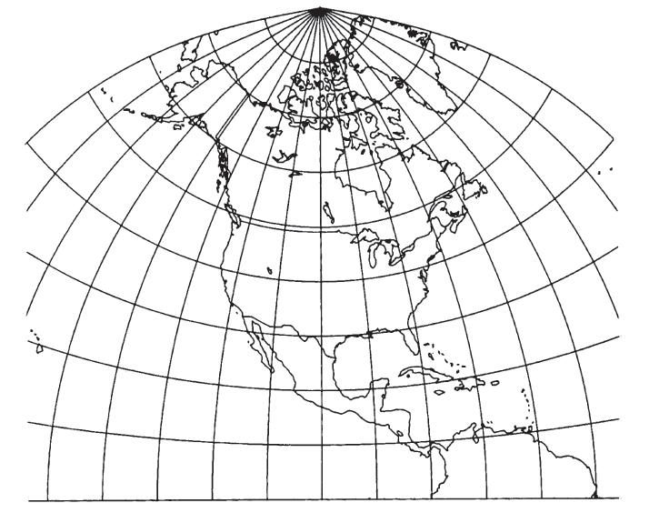

FEATURES #

The Polyconic projection (fig. 25) is neither equal-area nor conformal. Along the central meridian, however, it is both distortion free and true to scale. Each parallel is true to scale, but the meridians are lengthened by various amounts to cross each parallel at the correct position along the parallel, so that no parallel is standard in the sense of having conformality (or correct angles), except at the central meridian. Near the central meridian, which is the case with 7½-minute quadrangles, distortion is extremely small. The Polyconic projection is universal in that tables of rectangular coordinates may be used for any Polyconic projection of the same ellipsoid by merely applying the proper scale and central meridian. U.S. Coast and Geodetic Survey Special Publication No. 5 (1900) replaced tables published in 1884 and was often reprinted because of the universality of the projection (the Clarke 1866 is the reference ellipsoid). Polyconic quadrangle maps prepared to the same scale and for the same central meridian and ellipsoid will fit exactly from north to south. Since they are drawn in practice with straight meridians, they also fit east to west, but discrepancies will accumulate if mosaicking is attempted in both directions.

The parallels are all circular arcs, with the centers of the arcs lying along an extension of the straight central meridian, but these arcs are not concentric. Instead, as noted earlier, the radius of each arc is that of the circle developed from a cone tangent to the sphere or ellipsoid at the latitude. For the sphere, each parallel has a radius proportional to the cotangent of the latitude. For the ellipsoid, the radius is slightly different. The Equator is a straight line in either case. Along the central meridian, the parallels are spaced at their true intervals. For the sphere, they are therefore equidistant. Each parallel is marked off for meridians equidistantly and true to scale. The points so marked are connected by the curved meridians.

USAGE #

As geodetic and coastal surveying began in earnest during the 19th century, the Polyconic projection became a standard, especially for quadrangles. Most coastal charts produced by the Coast Survey and its successor during the 19th century were based on one or more variations of the Polyconic projection (Shalowitz, 1964, p. 138-141). The name of the projection appears on a later reprint of one of the first published USGS topographic quadrangles, which appeared in 1886. In 1904, the USGS published tables of rectangular coordinates extracted from an 1884 Coast and Geodetic Survey report. They were called “coordinates of curvature,” but were actually coordinates for the Polyconic projection, although the latter term was not used (Gannett, 1904, p. 37-48).

As a 1928 USGS bulletin of topographic instructions stated (Beaman, 1928, p. 163):

The topographic engineer needs a projection which is simple in construction, which can be used to represent small areas on any part of the globe, and which, for each small area to which it is applied, preserves shapes, areas, distances, and azimuths in their true relation to the surface of the earth. The polyconic projection meets all these needs and was adopted for the standard topographic map of the United States, in which the 1° quadrangle is the largest unit *** and the 15’ quadrangle is the average unit. *** Misuse of this projection in attempts to spread it over large areas – that is, to construct a single map of a large area-has developed serious errors and gross exaggeration of details. For example, the polyconic projection is not at all suitable for a single-sheet map of the United States or of a large State, although it has been so employed.

When coordinate plotters and published tables for the State Plane Coordinate System (SPCS) became available in the late 1950’s, the USGS ceased using the Polyconic for new maps, in favor of the Transverse Mercator or Lambert Conformal Conic projections used with the SPCS for the area involved. Some of the quadrangles prepared on one or the other of these projections have continued to carry the Polyconic designation, however.

The Polyconic projection was also used for the Progressive Military Grid for military mapping of the United States. There were seven zones, A-G, with central meridians every 8° west from long. 73° W. (zone A), each zone having an origin at lat. 40°30’ N. on the central meridian with coordinates $x= 1,000,000$ yards, $y =2,000,000$ yards (Deetz and Adams, 1934, p. 87-90). Some USGS quadrangles of the 1930’s and 1940’s display tick marks according to this grid in yards, and many quadrangles then prepared by the Army Map Service and sold by the USGS show a complete grid pattern. This grid was incorporated intact into the World Polyconic Grid (WPG) until both were superseded by the Universal Transverse Mercator grid (Mugnier, 1983).

While quadrangles based on the Polyconic provide low-distortion mapping of the local areas, the inability to mosaic these quadrangles in all directions without gaps makes them less satisfactory for a larger region. Quadrangles based on the SPCS may be mosaicked over an entire zone, at the expense of increased distortion.

For an individual quadrangle 7½ or 15 minutes of latitude or longitude on a side, the distance of the quadrangle from the central meridian of a Transverse Mercator zone or from the standard parallels of a Lambert Conformal Conic zone of the SPCS has much more effect than the type of projection upon the variation in measurement of distances on quadrangles based on the various projections. If the central meridians or standard parallels of the SPCS zones fall on the quadrangle, a change of projection from Polyconic to Transverse Mercator or Lambert Conformal Conic results in a difference of less than 0.001 mm in the measurement of the 700-800 mm diagonals of a 7½-minute quadrangle. If the quadrangle is near the edge of a zone, the discrepancy between measurements of diagonals on two maps of the same quadrangle, one using the Transverse Mercator or Lambert Conformal Conic projection and the other using the Polyconic, can reach about 0.05 mm. These differences are exceeded by variations in expansion and contraction of paper maps, so that these mathematical discrepancies apply only to comparisons of stable-base maps.

Actually, the central meridian of a 7½-minute Polyconic quadrangle may lie along the edge of the map, since 15-minute quadrangles were frequently cut and enlarged to achieve the less extensive coverage. This has a negligible effect upon the map geometry.

Before the Lambert became the projection for the 1:500,000 State base map series, a modified form of the Polyconic was used, but the details are unclear. The Polyconic was used for the base maps of Alaska until 1972. It has also been used for maps of the United States; but, as stated above, the distortion is excessive at the east and west coasts, and most current maps are drawn to either the Lambert or Albers Conic projections. There are several other modified Polyconic projections, in use or devised, including the Rectangular Polyconic and Bousfield’s modification used for northern Canada (Haines, 1981). The best known is that used for the International Map of the World, described on p. 131.

GEOMETRIC CONSTRUCTION #

Because of the simplicity of construction using universal tables with which the central meridian and each parallel may be marked off at true distances, the Polyconic projection was favored long after theoretically better projections became known in geodetic circles.

The Polyconic projection must be constructed with curved meridians and parallels if it is used for single-sheet maps of areas with east-west extent of several degrees. Then, however, the inherent distortion is excessive, and a different projection should be considered. For accurate topographic work, the coverage must remain so small that the meridians and parallels may ironically but satisfactorily be drawn as straight-line segments. Official USGS instructions of 1928 declared that

in actual practice on projections of small quadrangles, the parallels are not drawn as arcs of circles, but their intersections with the meridians are plotted from the computed x and y values, and the sections of the parallels between adjacent meridians are drawn as straight lines. In polyconic projections of quadrangles of 1° or smaller meridians may be drawn as straight lines, and in large-scale projections of small quadrangles in low latitudes both meridians and parallels may be drawn as straight lines. For example, the curvature of the parallels of a projection of a 15’ quadrangle on a scale of 1:48,000 in latitudes from 0° to 30° is so small that it can not be plotted, and for a 7½ quadrangle on a scale of 1:31,680 or larger the curvature can not be plotted at any latitude (Beaman, 1928, p. 167).

This instruction is essentially repeated in the 1964 edition (USGS, 1964, p. 12-13). The formulas given below are based on curved meridians.

FORMULAS FOR THE SPHERE #

The principles stated above lead to the following forward formulas for rectangular coordinates for the spherical form of the Polyconic projection, using radians (see numerical examples):

If $\phi$ is 0,

$$ x = R (\lambda - \lambda_0) \tag{ 7-1 } $$

$$ y=-R\phi_0 \tag{ 18-1 } $$

If $\phi$ is not 0,

$$ E = (\lambda - \lambda_0)\sin\phi \tag{ 18-2 } $$

$$ x = R\cot\phi\sin{E} \tag{ 18-3 } $$

$$ y = R[\phi-\phi_0+\cot\phi\,(1-\cos{E})] \tag{ 18-4 } $$

where $\phi_0$, is an arbitrary latitude (frequently the Equator) chosen for the origin of the rectangular coordinates at its intersection with $\lambda_0$, the central meridian. As with other conics and the Transverse Mercator, the Y axis coincides with the central meridian, y increasing northerly, and the X axis intersects perpendicularly at $\phi_0$, x increasing easterly. If $(\lambda - \lambda_0)$ exceeds the range -+180°, 360° must be added or subtracted to place it within the range. For the scale factor $h$ along the meridians (Adams, 1919, p. 144-147):

$$ h = (1-\cos^2\phi\cos{E})/(\sin^2\phi\cos{D}) \tag{ 18-5 } $$

where

$$ D = \arctan[(E-\sin{E})/(\sec^2\phi-\cos{E})] \tag{ 18-6 } $$

If $\phi$ is 0, this is indeterminate, but $h$ is then $[1+ (\lambda - \lambda_0)^2/2]$. In all cases, the scale factor k along any parallel is 1.0.

The inverse formulas for the sphere are given here in the form of a Newton-Raphson approximation, which converges to any desired accuracy after several iterations, except that if $|\lambda - \lambda_0|>90°$, a rarely used range, this iteration does not converge, and if $y = -R\phi_0$, it is indeterminate. In the latter case, however,

$$ \phi = 0 $$

$$ \lambda = x/R + \lambda_0 \tag{ 7-5 } $$

Otherwise, if $y \ne -R\phi_0$, calculations are made in this order:

$$ A = \phi_0 + y/R \tag{ 18-7 } $$

$$ B = x^2/R^2+A^2 \tag{ 18-8 } $$

Using an initial value of $\phi_n=A$, $\phi_{n+1}$, is found from equation (18-9),

$$ \begin{align} \phi_{n+1} =& \phi_n-[A(\phi_n\tan\phi_n+1)-\phi_n-1/2(\phi_n^2+B)\tan\phi_n]/ \\ & [(\phi_n-A)/\tan\phi_n-1] \end{align} \tag{ 18-9 } $$

The new trial value of $\phi_{n+1}$ is successively substituted in place of $\phi_n$, until $\phi_{n+1}$ differs from $\phi_n$ , by less than a predetermined convergence limit. Then $\phi = \phi_{n+1}$ as finally determined.

$$ \lambda = [\arcsin(x\tan\phi/R)]/\sin\phi+\lambda_0 \tag{ 18-10 } $$

If $\phi =\pm 90^\circ$, equation (18-10) is indeterminate, but $\lambda$ may be given any value, such $\lambda_0$.

FORMULAS FOR THE ELLIPSOID #

The forward formulas for the ellipsoidal form of the Polyconic projection are only a little more complicated than those for the sphere. These formulas are theoretically exact. They are adapted from formulas given by the Coast and Geodetic Survey (1946, p. 4) (see numerical examples): If $\phi$ is 0,

$$ x = a (\lambda - \lambda_0) \tag{ 7-6 } $$

$$ y=M_0 \tag{ 18-11 } $$

If $\phi$ is not 0,

$$ E = (\lambda - \lambda_0)\sin\phi \tag{ 18-2 } $$

$$ x= N\cot\phi\sin{E} \tag{ 18-12 } $$

$$ y = M - M_0+N\cot\phi(1-\cos{E}) \tag{ 18-13 } $$

where

$$ \begin{align} M = a[&(1-e^2/4-3e^4/64-5e^6/256-\dots)\phi \\ -&(3e^2/8+3e^4/32+45e^6/1024+\dots)\sin{2\phi} \\ +&(15e^4/256+45e^6/1024+\dots)\sin{4\phi} - (35e^6/3072+\dots)\sin{6\phi}+\dots] \end{align} \tag{ 3-21 } $$

$$ N = a/(1-e^2\sin^2{\phi})^{1/2} \tag{ 4-20 } $$

and $M_0$ is found from equation (3-21) by using $\phi_0$ for $\phi$ and $M_0$ for $M$, with $\phi_0$ the latitude of the origin of rectangular coordinates at its intersection with central meridian $\lambda_0$. See the spherical formulas for the orientation of axes. The value of $(\lambda-\lambda_0$) must be adjusted by adding or subtracting 360° if necessary to fall within the range of $\pm180°$. For scale factor h along the meridians (k = 1.0 along the parallels):
If $\phi$ is zero,

$$ h= [M'+1/2(\lambda-\lambda_0)^2]/(1-e^2) \tag{ 18-14 } $$

If $\phi$ is not zero (Adams, 1919, p. 144-146)

$$ h = [1-e^2+2(1-e^2\sin^2\phi)\sin^2½E/\tan^2\phi]/[(1-e^2)\cos{D}] \tag{ 18-15 } $$

where

$$ D = \arctan\{(E-\sin{E})[\sec^2\phi-\cos{E}-e^2\sin^2\phi/(1-e^2\sin^2\phi)]\} \tag{ 18-16 } $$

$$ \begin{align} M' =& 1-e^2/4-3e^4/64-5e^6/256-\dots \\ &-2(3e^2/8+3e^4/32+45e^6/1024+\dots)\cos{2\phi} \\ &+4(15e^4/256+45e^6/1024+\dots)\cos{4\phi} \\ &-6(35e^6/3072+\dots)\cos{6\phi}+\dots \end{align} \tag{ 18-17 } $$

For improved computational efficiency using this series, see p. 19.

As with the inverse spherical formulas, the inverse ellipsoidal formulas are given in a Newton-Raphson form, converging to any desired degree of accuracy after several iterations. As before, if $|\lambda-\lambda_0|>90^\circ$, this iteration does not converge, but the projection should not be used in that range in any case. The formulas may be calculated in the following order, given $a, e, \phi_0, \lambda_0, x,$ and $y$. First $M_0$ is calculated from equation (3-21) above, as in the forward case, with $\phi_0$ for $\phi$ and $M_0$ for $M$.

If $y=M_0$, the iteration is not applicable, but

$$ \phi = 0 $$

$$ \lambda = x/a + \lambda_0 \tag{ 7-12 } $$

If $y \ne -M_0$, the calculation is as follows:

$$ A=(M_0+y)/a \tag{ 18-18 } $$

$$ B=x^2/a^2+A^2 \tag{ 18-19 } $$

Using an initial value of $\phi_n=A$, the following calculations are made:

$$ C=(1-e^2\sin^2{\phi_n})^{1/2}\tan{\phi_n} \tag{ 18-20 } $$

Then $M_n$, and $M_n’$ are found from equations (3-21) and (18-17) above, using $\phi_n$, for $\phi$, $M_n$ , for $M$, and $M_n’$ for $M’$. Let $M_a = M_n/a$.

$$ \begin{align} \phi_{n+1} =\;& \phi_n-[A(C M_a+1)-M_a-(M_a^2+B)C/2]/ \\ &[e^2\sin{2\phi_n}(M_a^2+B-2A M_a)/4C \\ &+ (A-M_a)(C M_n'-2/\sin{2\phi_n}) -M_n'] \end{align} \tag{ 18-21 } $$

Each value of $\phi_{n+1}$ is substituted in place of $\phi_n$, and $C, M_n, M_n’$, and $\phi_{n+1}$ are recalculated from equations (18-20), (3-21), (18-17), and (18-21), respectively. This process is repeated until $\phi_{n+1}$ varies from $\phi_n$, by less than a predetermined convergence value. Then $\phi$ equals the final $\phi_{n+1}$.

$$ \lambda =[\arcsin(x C/a)]/\sin\phi+\lambda_0 \tag{ 18-22 } $$

using the $C$ calculated for the last $\phi_n$, from equation (18-20). If $\phi=\pm90°$, $\lambda$ is indeterminate, but may be given any value.

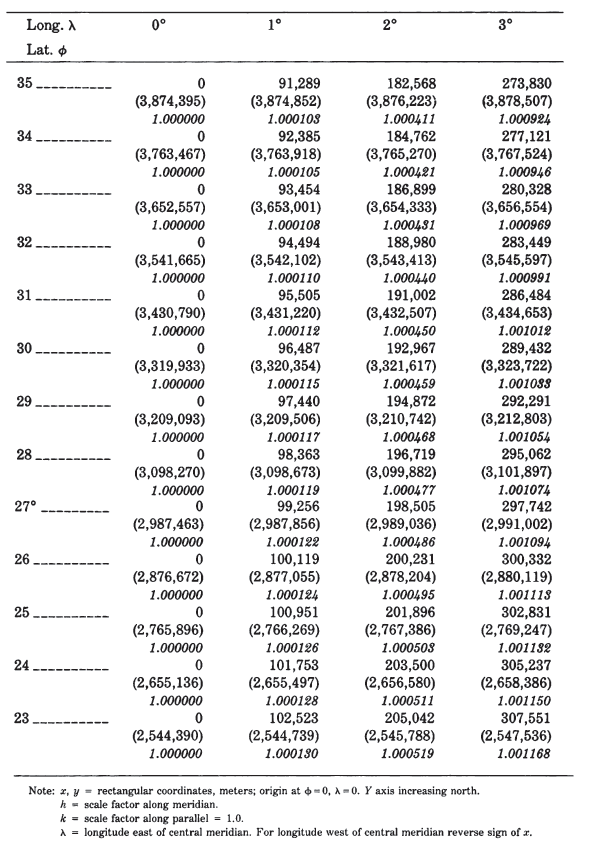
Table 19 lists rectangular coordinates for a band 3° on either side of the central meridian for the ellipsoid extending from lat. 23° to 50° N. Figure 25 shows the graticule applied to a map of North America.

TABLE 19.— Polyconic Projection: Rectangular coordinates for the Clarke 1866 ellipsoid — **TABLE 19**.— Polyconic Projection: Rectangular coordinates for the Clarke 1866 ellipsoid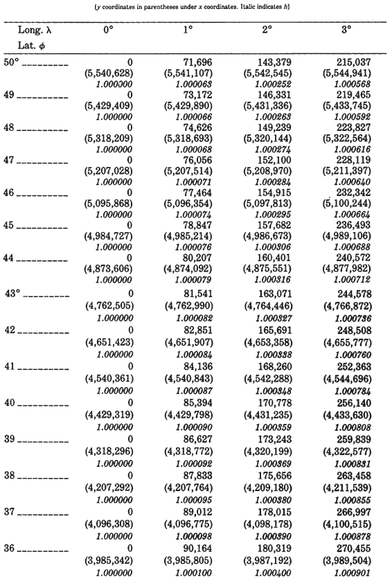

MODIFIED POLYCONIC FOR THE INTERNATIONAL MAP OF THE WORLD #

A modified Polyconic projection was devised by Lallemand of France and in 1909 adopted by the International Map Committee (IMC) in London as the basis for the 1:1,000,000-scale International Map of the World (IMW) series. Used for sheets 6° of longitude by 4° of latitude between lats. 60° N. and 60° S., 12° of longitude by 4° of latitude between lats. 60° and 76° N. or S., and 24° by 4° between lats. 76° and 84° N. or S., the projection differs from the ordinary Polyconic in two principal features: All meridians are straight, and there are two meridians (2° east and west of the central meridian on sheets between lats. 60° N. & S.) that are made true to scale. Between lats. 60° & 76° N. and S., the meridians 4° east and west are true to scale, and between 76° & 84°, the true-scale meridians are 8° from the central meridian (United Nations, 1963, p. 22-23; Lallemand, 1911, p. 559).

The top and bottom parallels of each sheet are nonconcentric circular arcs constructed with radii of $N\cot\phi$, where $N = a/(1- e^2\sin^2\phi)^{1/2}$. These radii are the same as the radii on the regular Polyconic for the ellipsoid, and the arcs of these two parallels are marked off true to scale for the straight meridians. The two parallels, however, are spaced from each other according to the true scale along the two standard meridians, not according to the scale along the central meridian, which is slightly reduced. The approximately 440 mm true length of the central meridian at the map scale is thereby reduced by 0.270 to 0.076 mm, depending on the latitude of the sheet. Other parallels of lat. $\phi$ are circular arcs with radii $N\cot\phi$, intersecting the meridians which are true to scale at the correct points. The parallels strike other meridians at geometrically fixed locations which slightly deviate from the true scale on meridians as well as parallels. With this modified Polyconic, as with USGS quadrangles based on the rectified Polyconic, adjacent sheets exactly fit together not only north to south, but east to west. There is still a gap when mosaicking in all directions, in that there is a gap between each diagonal sheet and either one or the other adjacent sheet.

In 1962, a U.N. conference on the IMW adopted the Lambert Conformal Conic and Polar Stereographic projections to replace the modified Polyconic (United Nations, 1963, p. 9-10). The USGS has prepared a number of sheets for the IMW series over the years according to the projection officially in use at the time.

FORMULAS FOR THE IMW MODIFIED POLYCONIC #

Since the projection was designed solely for this series, the formulas below are based on the ellipsoid. They were derived in 1982 (Snyder, 198213). The following symbols are used in these formulas:

$$ \begin{align} a = &\text{ semimajor axis on the given reference ellipsoid} \\ C = &\text{ distance on the map of latitude $\phi$ from latitude measured along} \\ &\text{ the central meridian of longitude $\lambda$.} \\ C_2 = &\text{ distance on the map of latitude $\phi_2$ from latitude $\phi_1$, measured along} \\ &\text{ the central meridian of longitude $\lambda$} \\ e = &\text{ eccentricity of the given reference ellipsoid} \\ M = &\text{ distance on the ellipsoid along any meridian from the Equator to }\phi \\ M_2 = &\text{ ditto for } \phi_2 \\ M_1 = &\text{ ditto for } \phi_1 \\ R = &\text{ radius of circular arc for latitude $\phi$ as shown on map} \\ (x,y) = &\text{ rectangular coordinates, with the origin at the intersection of }\phi_1, \\ &\text{ with $\lambda_0$, the y axis coinciding with the meridian of longitude } \lambda_0, \\ &\text{ y increasing northerly, and the x axis perpendicular, x increasing easterly} \\ \lambda = &\text{ longitude of any meridian (east longitude is positive)} \\ \lambda_0 = &\text{ longitude of central meridian} \\ \lambda_1 = &\text{ longitude of true-to-scale meridian east of the central meridian, } 2^\circ \\ &\text{ more than $\lambda$, for most quadrangles }\\ \phi = &\text{ any geodetic (or geographic) latitude on the quadrangle map}\\ \phi_2 = &\text{ geodetic latitude of the northernmost parallel of a given quadrangle}\\ &\text { map (north latitude is positive)}\\ \phi_1 = &\text{ geodetic latitude of the southernmost parallel of the quadrangle map} \end{align} $$

Care must be taken to use radians wherever angles are used without trigonometric functions. The following constants apply to the entire map, given $a, e, \phi_1, \phi_2, \lambda_1,$ and $\lambda_0$:

$$ x_n = R_n\sin{F_n} \tag{ 18-23 } $$

$$ y_1 = R_1(1-\cos{F_1}) \tag{ 18-24 } $$

$$ T_2 = R_2(1-\cos{F_2}) \tag{ 18-25 } $$

where $n = 1$ and $2$, and

$$ R_n = a\cot{\phi_n}/(1-e^2\sin^2\phi_n)^{1/2} \tag{ 18-26 } $$

$$ F_n = (\lambda_1-\lambda_0)\sin\phi_n \tag{ 18-27 } $$

with subscripts as required above, but if $\phi_n = 0, R_n$ is infinite and equations (18-23) and (18-24) are indeterminate, but $y_1 = 0, T_2 = 0,$ and

$$ x_n = a(\lambda_1 - \lambda_0) \tag{ 18-23a } $$

Also for the entire map,

$$ y_2 = [(M_2-M_1)^2-(x_2-x_1)^2]^{1/2}+y_1 \tag{ 18-28 } $$

$$ C_2 = y_2 - T_2 \tag{ 18-29 } $$

$$ P = (M_2 y_1-M_1 y_2)/(M_2-M_1) \tag{ 18-30 } $$

$$ Q = (y_2-y_1)/(M_2-M_1) \tag{ 18-31 } $$

$$ P' = (M_2 x_1-M_1 x_2)/(M_2-M_1) \tag{ 18-32 } $$

$$ Q' = (x_2-x_1)/(M_2-M_1) \tag{ 18-33 } $$

where

with subscripts as required above.

The following values are calculated for each point, given $\phi$ and $\lambda$; to find $x$ and $y$:

$$ x_a = P'+Q'M \tag{ 18-34 } $$

$$ y_a = P'+Q M \tag{ 18-35 } $$

$$ C = y_a-R\pm(R^2-x_a^2)^{1/2} \tag{ 18-36 } $$

where the $\pm$ takes the same sign as $\phi$. If $\phi = 0$, equation (18-36) is indeterminate, but $C = 0$. $M$ and $R$ are found from (3-21) and (18-26), respectively, omitting subscripts $n$. Then

$$ x_b = R_2\sin[(\lambda-\lambda_0)\sin\phi_2] \tag{ 18-37 } $$

$$ y_b = C_2 + R_2\{1-\cos[(\lambda-\lambda_0)\sin\phi_2]\} \tag{ 18-38 } $$

$$ x_c = R_1\sin[(\lambda-\lambda_0)\sin\phi_1] \tag{ 18-39 } $$

$$ y_c = R_1\{1-\cos[(\lambda-\lambda_0)\sin\phi_1]\} \tag{ 18-40 } $$

but if $\phi_2=0,$

$$ x_b = a(\lambda-\lambda_0) \tag{ 18-37a } $$

$$ y_b = C_2 \tag{ 18-38a } $$

or if $\phi_1 = 0,$

$$ x_c = a(\lambda-\lambda_0) \tag{ 18-39a } $$

$$ y_c = 0 \tag{ 18-40a } $$

Then

$$ D = (x_b-x_c)/(y_b-y_c) \tag{ 18-41 } $$

$$ B = x_c + D(C+R-y_c) \tag{ 18-42 } $$

$$ x = \{B\pm D[R^2(1+D^2)-B^2]^{1/2}\}/(1+D^2) \tag{ 18-43 } $$

$$ y = C + R \pm (R^2-x^2)^{1/2} \tag{ 18-44 } $$

where the $\pm$ in (18-43) and (18-44) takes the sign opposite that of $\phi$. If $\phi = 0, B$ and $R$ are infinite, but

$$ x = a(\lambda-\lambda_0) \tag{ 18-45 } $$

$$ y = C \tag{ 18-46 } $$

For the inverse formulas for the IMW Modified Polyconic, given $a, e, \phi_2, \phi_1, \lambda_1, \lambda_0, x$ and $y$, to find $\phi$ and $\lambda$:

Constants are calculated: $x_1, x_2, y_1, y_2, C_2, P, Q, P’,$ and $Q’$ from above equations (18-23) through (18-33) and (3-21).
A first trial $(\phi, \lambda)$, called $(\phi_{t_1}, \lambda_{t_1})$ are calculated:
$$ \phi_{t_1} = \phi_2 \tag{ 18-47 } $$
$$ \lambda_{t_1} = [x/(a\cos\phi_{t_1})]+\lambda_0 \tag{ 18-48 } $$
The first test values of $(x, y)$, called $(x_{t_1}, y_{t_1})$, are calculated from $(\phi_{t_1}, \lambda_{t_1})$, using the latter as $(\phi,\lambda)$ in equations (18-34) through (18-46).
Test values $(x_{t_1}, y_{t_1})$ are used with the given $(x, y)$ to adjust $(\phi_{t_1}, \lambda_{t_1})$, to provide second trial values of $(\phi_{t_2}, \lambda_{t_2})$:
$$ \phi_{t_2}=[(\phi_{t_1}-\phi_1)(y-y_c)/(y_{t_1}-y_c)] +\phi_1 \tag{ 18-49 } $$
$$ \lambda_{t_2} = [(\lambda_{t_1}-\lambda_0)x/x_{t_1}] +\lambda_0 \tag{ 18-50 } $$
Step 3 is repeated, but using $(\phi_{t_2}, \lambda_{t_2})$ as $(\phi, \lambda)$ to obtain $(x_{t_2}, y_{t_2})$. Step 4 is then repeated, replacing subscripts $(t_l, t_2)$ with $(t_2, t_3)$, respectively. Steps 3 and 4 are repeated, changing subscripts, until the final $(x_{t_n}, y_{t_n})$ vary from $(x, y)$, respectively, by an acceptable total absolute error, such as 1 meter (0.001 mm at map scale).

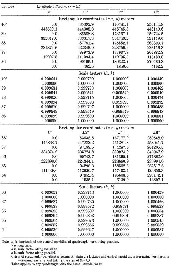
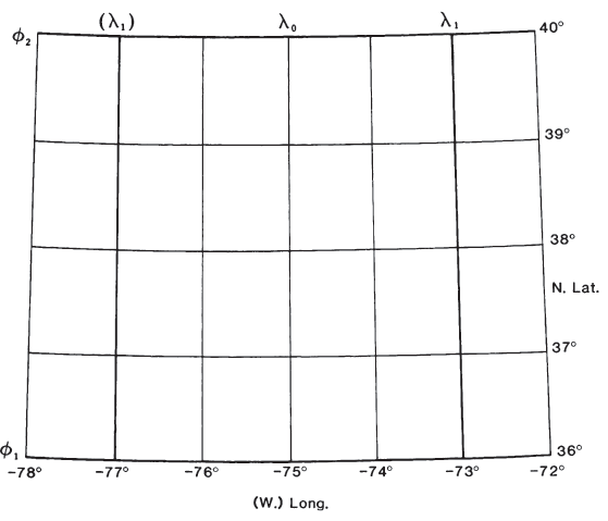
Table 20 provides samples of rectangular coordinates calculated for each degree of typical mid-latitude and far-northern quadrangles. In addition, scale factors $h$ (along the meridian) and $k$ (along the parallel) are shown for the same graticules.

TABLE 20.— Modified Polyconic projection for IMW: Rectangular coordinates for the International ellipsoid — **TABLE 20**.— Modified Polyconic projection for IMW: Rectangular coordinates for the International ellipsoid

The scale factors were calculated by comparing rectangular coordinates 0.01° of latitude apart at constant longitude with the true distances, for $h$, and a similar change in longitude at constant latitude, for $k$, rather than analytically. The linear scale error is seen to change less than about 0.06 percent throughout the quadrangle; the scale factor along any given parallel is almost constant, while a given meridian varies up to 0.015 percent in scale. The table is based on the International ellipsoid or spheroid, although the skeletal tables showing rectangular coordinates of parallels $\phi_1$, and $\phi_2$ and published in earlier technical papers are based on an ellipsoid with a semimajor axis of 6378.24 km and semiminor axis of 6356.56 km. Figure 26 illustrates a typical graticule.

FIGURE 26.— Typical IMW quadrangle graticule - modified Polyconic projection drawn to scale. Parallels are nonconcentric circular arcs; meridians are straight. Lines of true scale are shown heavy. Standard projection for the International Map of the World Series (1:1,000,000-scale) until 1962 — **FIGURE 26**.— Typical IMW quadrangle graticule - modified Polyconic projection drawn to scale. Parallels are nonconcentric circular arcs; meridians are straight. Lines of true scale are shown heavy. Standard projection for the International Map of the World Series (1:1,000,000-scale) until 1962