19. BONNE PROJECTION #
SUMMARY #
- Pseudoconical.
- Central meridian is a straight line. Other meridians are complex curves.
- Parallels are concentric circular arcs, but the poles are points.
- Scale is true along the central meridian and along all parallels.
- No distortion along the central meridian and along the standard parallel.
- Used for atlas maps of continents and for topographic mapping of some countries.
- Sinusoidal projection is equatorial limiting form of Bonne projection.
- Used considerably by Bonne in mid-18th century, but developed by others during the early 16th century.
HISTORY #
The name of Rigobert Bonne (1727-1795), a French geographer, is almost universally applied to an equal-area projection which has been used for both large- and small-scale mapping during the past 450 years. During the late 19th and early 20th centuries, the most conspicuous use of the Bonne projection was for maps of continents in atlases.
The Italian Bernardus Sylvanus’ world map of 1511 closely approaches the Bonne projection, since its meridians are almost equally spaced along the equidistant and concentric circular parallels. De l’Isle and Coronelli used the Bonne principle for maps of about 1700. Bonne used the projection most notably for a 1752 maritime atlas of the coast of France (Reignier, 1957, p. 164). Continental maps of Europe and Asia appeared on this projection by 1763, and the ellipsoidal version replaced the Cassini projection for French topographic mapping beginning in 1803.
For maps of continents, the Bonne was preceded by its polar limiting form, a cordiform (heart-shaped) world map devised by Johannes Stabius and given wider notice by Johannes Werner about 1514. The Werner projection, as it is usually called, was used in the late 16th century for maps of Asia and Africa by Mercator and Abraham Ortelius, but the “Bonne” projection has less distortion because its projection center is at the center of the region being mapped instead of at the pole. Eventually the Werner projection was made obsolete by the Bonne.
FEATURES AND USAGE #
Like the Equidistant Conic with one standard parallel, the Bonne projection (fig. 27) has concentric circular arcs for parallels of latitude. They are equally spaced on the spherical form and spaced in proportion to the true distance along a meridian on the ellipsoidal form. The chosen standard parallel is given its true curvature on the map by making the radius of its circular arc equal to the distance between the parallel and the apex of a cone tangent at the parallel. FIGURE 27.— Bonne projection with central parallel at lat. 40° N. Called a pseudoconic projection, this is equal-area and has no distortion along central meridian or central parallel. Popular in atlases for maps of continents until mid-20th century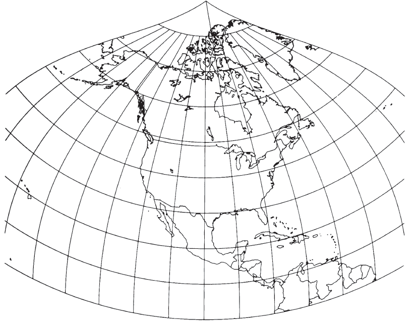
The combination of curved meridians and concentric circular arcs for parallels has led to the classification of “pseudoconic” for the Bonne projection and for the polar limiting case, the Werner projection, on which the North Pole is the equivalent of the standard parallel. The limiting case with the Equator as the standard parallel is the Sinusoidal, a “pseudocylindrical” projection to be discussed later; the formulas must be changed in this case since the parallels of latitude are straight. Modifications to the Bonne projection, in some cases resulting in nonequal-area projections, were presented by Nell of Germany in 1890 and by Solov’ev of the Soviet Union in the 1940’s (Maling, 1960, p. 295-296).
Many atlases of the 19th and early 20th centuries utilized the Bonne projection to show North America, Europe, Asia, and Australia, while the Sinusoidal (as the equatorial Bonne) was used for South America and Africa. The Lambert Azimuthal Equal-Area projection is now generally used by Rand McNally & Co. and Hammond Inc. for maps of continents, while the National Geographic Society prefers its own Chamberlin Trimetric projection for this purpose.
Large-scale use of the Bonne projection for topographic mapping, originally introduced by France, is current chiefly in portions of France, Ireland, Morocco, and some countries in the eastern Mediterranean area (Clifford J. Mugnier, written commun., 1985).
FORMULAS FOR THE SPHERE #
The principles stated above lead to the following forward formulas for rectangular coordinates of the spherical form of the Bonne projection, given $R, \phi_1, \lambda_0, \phi$ and $\lambda$, and using radians in equation (19-1),
The inverse formulas for the sphere, given $R, \phi_1, \lambda_0, x$, and $y$, to find $(\phi, \lambda)$:
FORMULAS FOR THE ELLIPSOID #
For the forward formulas, given $a, e, \phi_1, \lambda_0, \phi$, and $\lambda$, to find $x$ and $y$, the following are calculated in order:
For the inverse formulas for the ellipsoid, given $a, e, \phi_1, \lambda_0, x$ and $y$, to find $\phi$ and $\lambda$, first $m_1$, and $M_1$ are calculated as in the forward case from equations (14-15) and (3-21) above. The following are then calculated in order: