CONIC MAP PROJECTIONS #
Cylindrical projections are used primarily for complete world maps, or for maps along narrow strips of a great circle arc, such as the Equator, a meridian, or an oblique great circle. To show a region for which the greatest extent is from east to west in the temperate zones, conic projections are usually preferable to cylindrical projections.
Normal conic projections are distinguished by the use of arcs of concentric circles for parallels of latitude and equally spaced straight radii of these circles for meridians. The angles between the meridians on the map are smaller than the actual differences in longitude. The circular arcs may or may not be equally spaced, depending on the projection. The Polyconic projection and oblique conic projections have characteristics different from these.
The name “conic” originates from the fact that the more elementary conic projections may be derived by placing a cone on the top of a globe representing the Earth, the apex or tip in line with the axis of the globe, and the sides of the cone touching or tangent to the globe along a specified “standard” latitude which is true to scale and without distortion (see fig. 1). Meridians are drawn on the cone from the apex to the points at which the corresponding meridians on the globe cross the standard parallel. Other parallels are then drawn as arcs centered on the apex in a manner depending on the projection. If the cone is cut along one meridian and unrolled, a conic projection results. A secant cone results if the cone cuts the globe at two specified parallels. Meridians and parallels can be marked on the secant cone somewhat as above, but this will not result in any of the common conic projections with two standard parallels. They are derived from various desired scale relationships instead, and the spacing of the meridians as well as the parallels is not the same as the projection onto a secant cone.
There are three important classes of conic projections: the equidistant (or simple), the conformal, and the equal-area. The Equidistant Conic, with parallels equidistantly spaced, originated in a rudimentary form with Claudius Ptolemy. It eventually developed into commonly used present-day forms which have one or two standard parallels selected for the area being shown. It is neither conformal nor equal-area, but north-south scale along all meridians is correct, and the projection can be a satisfactory compromise for errors in shape, scale, and area, especially when the map covers a small area. It is primarily used in the spherical form, although the ellipsoidal form is available and useful. The USGS uses the Equidistant Conic in an approximate form for a map of Alaska, identified as a “Modified Transverse Mercator” projection, and also in the limiting equatorial form: the Equidistant Cylindrical. Both are described earlier.
The Lambert Conformal Conic projection with two standard parallels is used frequently for large- and small-scale maps. The parallels are more closely spaced near the center of the map. The Lambert has also been used slightly in the oblique form. The Albers Equal-Area Conic with two standard parallels is used for sectional maps of the U.S. and for maps of the conterminous United States. The Albers parallels are spaced more closely near the north and south edges of the map. There are some conic projections, such as perspective conics, which do not fall into any of these three categories, but they are rarely used.
The useful conic projections may be geometrically constructed only in a limited sense, using polar coordinates which must be calculated. After a location is chosen, usually off the final map, for the center of the circular arcs which will represent parallels of latitude, meridians are constructed as straight lines radiating from this center and spaced from each other at an angle equal to the product of the cone constant times the difference in longitude. For example, if a 10° graticule is planned, and the cone constant is 0.65, the meridian lines are spaced at 10° times 0.65 or 6.5°. Each parallel of latitude may then be drawn as a circular arc with a radius previously calculated from formulas for the particular conic projection.
14. ALBERS EQUAL-AREA CONIC PROJECTION #
SUMMARY #
- Conic.
- Equal-Area.
- Parallels are unequally spaced arcs of concentric circles, more closely spaced at the north and south edges of the map.
- Meridians are equally spaced radii of the same circles, cutting parallels at right angles.
- There is no distortion in scale or shape along two standard parallels, normally, or along just one.
- Poles are arcs of circles.
- Used for equal-area maps of regions with predominant east-west expanse, especially the conterminous United States.
- Presented by Albers in 1805.
HISTORY #
One of the most commonly used projections for maps of the conterminous United States is the equal-area form of the conic projection, using two standard parallels. This projection was first presented by Heinrich Christian Albers (1773-1833), a native of Luneburg, Germany, in a German periodical of 1805 (Albers, 1805; Bonacker and Anliker, 1930). The Albers projection was used for a German map of Europe in 1817, but it was promoted for maps of the United States in the early part of the 20th century by Oscar S. Adams of the Coast and Geodetic Survey as “an equal-area representation that is as good as any other and in many respects superior to all others” (Adams, 1927, p. 1).
FEATURES AND USAGE #
The Albers is the projection exclusively used by the USGS for sectional maps of all 50 States of the United States in the National Atlas of 1970, and for other U.S. maps at scales of 1:2,500,000 and smaller. The latter maps include the base maps of the United States issued in 1961, 1967, and 1972, the Tectonic Map of the United States (1962), and the Geologic Map of the United States (1974), all at 1:2,500,000. The USGS has also prepared a U.S. base map at 1:3,168,000 (1 inch = 50 miles).
Like other normal conics, the Albers Equal-Area Conic projection (fig. 20) has concentric arcs of circles for parallels and equally spaced radii as meridians. The parallels are not equally spaced, but they are farthest apart in the latitudes between the standard parallels and closer together to the north and south. The pole is not the center of the circles, but is normally an arc itself.
FIGURE 20.— Albers Equal-Area Conic projection, with standard parallels 20° and 60° N. This illustration includes all of North America to show the change in spacing of the parallels. When used for maps of the 48 conterminous States standard parallels are 29.5° and 45.5° N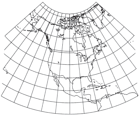
If the pole is taken as one of the two standard parallels, the Albers formulas reduce to a limiting form of the projection called Lambert’s Equal-Area Conic (not discussed here, and not to be confused with his Conformal Conic, to be discussed later). If the pole is the only standard parallel, the Albers formulas simplify to provide the polar aspect of the Lambert Azimuthal Equal-Area (discussed later). In both of these limiting cases, the pole is a point. If the Equator is the one standard parallel, the projection becomes Lambert’s Cylindrical Equal-Area (discussed earlier), but the formulas must be modified. None of these extreme cases applies to the normal use of the Albers, with standard parallels in the temperate zones, such as usage for the United States.
Scale along the parallels is too small between the standard parallels and too large beyond them. The scale along the meridians is just the opposite, and in fact the scale factor along meridians is the reciprocal of the scale factor along parallels, to maintain equal area. An important characteristic of all normal conic projections is that scale is constant along any given parallel.
To map a given region, standard parallels should be selected to minimize variations in scale. Not only are standard parallels correct in scale along the parallel; they are correct in every direction. Thus, there is no angular distortion, and conformality exists along these standard parallels, even on an equal-area projection. They may be on opposite sides of, but not equidistant from, the Equator. Deetz and Adams (1934, p. 79, 91) recommended in general that standard parallels be placed one-sixth of the displayed length of the central meridian from the northern and southern limits of the map. Hinks (1912, p. 87) suggested one-seventh instead of one-sixth. Others have suggested selecting standard parallels of conics so that the maximum scale error (1 minus the scale factor) in the region between them is equal and opposite in sign to the error at the upper and lower parallels, or so that the scale factor at the middle parallel is the reciprocal of that at the limiting parallels. Tsinger in 1916 and Kavrayskiy in 1934 chose standard parallels so that least-square errors in linear scale were minimal for the actual land or country being displayed on the map. This involved weighting each latitude in accordance with the land it contains (Maling, 1960, p. 263-266).
The standard parallels chosen by Adams for Albers maps of the conterminous United States are lats. 29.5° and 45.5°N. These parallels provide “for a scale error slightly less than 1 per cent in the center of the map, wit.h a maximum of 1¼ per cent along the northern and southern borders” (Deetz and Adams, 1934, p. 91). For maps of Alaska, the chosen standard parallels are lats. 55° and 65°N., and for Hawaii, lats. 8° and 18°N. In the latter case, both parallels are south of the islands, but they were chosen to include maps of the more southerly Canal Zone and especially the Philippine Islands. These parallels apply to all maps prepared by the USGS on the Albers projection, originally using Adams’s published tables of coordinates for the Clarke 1866 ellipsoid (Adams, 1927).
Without measuring the spacing of parallels along a meridian, it is almost impossible to distinguish an unlabeled Albers map of the United States from other conic forms. It is only when the projection is extended considerably north and south, well beyond the standard parallels, that the difference is apparent without scaling.
Since meridians intersect parallels at right angles, it may at first seem that there is no angular distortion. However, scale variations along the meridians cause some angular distortion for any angle other than that between the meridian and parallel, except at the standard parallels.
FORMULAS FOR THE SPHERE #
The Albers Equal-Area Conic projection may be constructed with only one standard parallel, but it is nearly always used with two. The forward formulas for the sphere are as follows, to obtain rectangular or polar coordinates, given $R, \phi_1, \phi_2, \phi_0, \lambda_0, \phi$, and $\lambda$ (see numerical examples):
The Y axis lies along the central meridian $\lambda_0$, $y$ increasing northerly. The X axis intersects perpendicularly at $\phi_0$, $x$ increasing easterly. If $(\lambda - \lambda_0)$ exceeds the range $\pm180°$, 360° should be added or subtracted to place it within the range. Constants $n, C$, and $\rho_0$ apply to the entire map, and thus need to be calculated only once. If only one standard parallel 4, is desired (or if $\phi_1=\phi_2$), $n=\sin\phi_1$. By contrast, a geometrically secant cone requires a cone constant $n$ of $\sin[(\phi_1+\phi_2)/2]$, slightly but distinctly different from equation (14-6). If the projection is designed primarily for the Northern Hemisphere, $n$ and $\rho$ are positive. For the Southern Hemisphere, they are negative. The scale along the meridians, using equation (4-4),
For the inverse formulas for the sphere, given $R, \phi_1, \phi_2, \phi_0, \lambda_0, x$, and $y$: $n, C$ and $\rho$, are calculated from equations (14-6), (14-5), and (14-3a), respectively. Then,
FORMULAS FOR THE ELLIPSOID #
The formulas displayed by Adams and most other writers describing the ellipsoidal form include series, but the equations may be expressed in closed forms which are suitable for programming, and involve no numerical integration or iteration in the forward form. Nearly all published maps of the United States based on the Albers use the ellipsoidal form because of the use of tables for the original base maps. (Adams, 1927, p. 1-7; Deetz and Adams, 1934, p. 93-99; Snyder, 1979a, p. 71). Given $a, e, \phi_1, \phi_2, \phi_0, \lambda_0, \phi$, and $\lambda$ (see numerical examples):
For the inverse formulas for the ellipsoid, given $a, e, \phi_1, \phi_2. \phi_0, \lambda_0, x$, and $y$: $n, C$, and $\rho_0$ are calculated from equations (14-14), (14-13), and (14-12a); respectively. Then,
Instead of the iteration, a series may be used for the inverse ellipsoidal formulas:
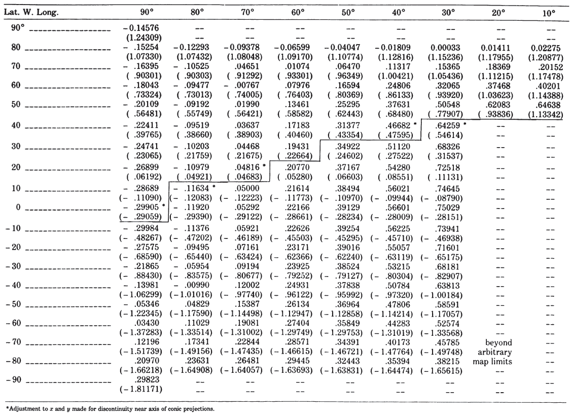
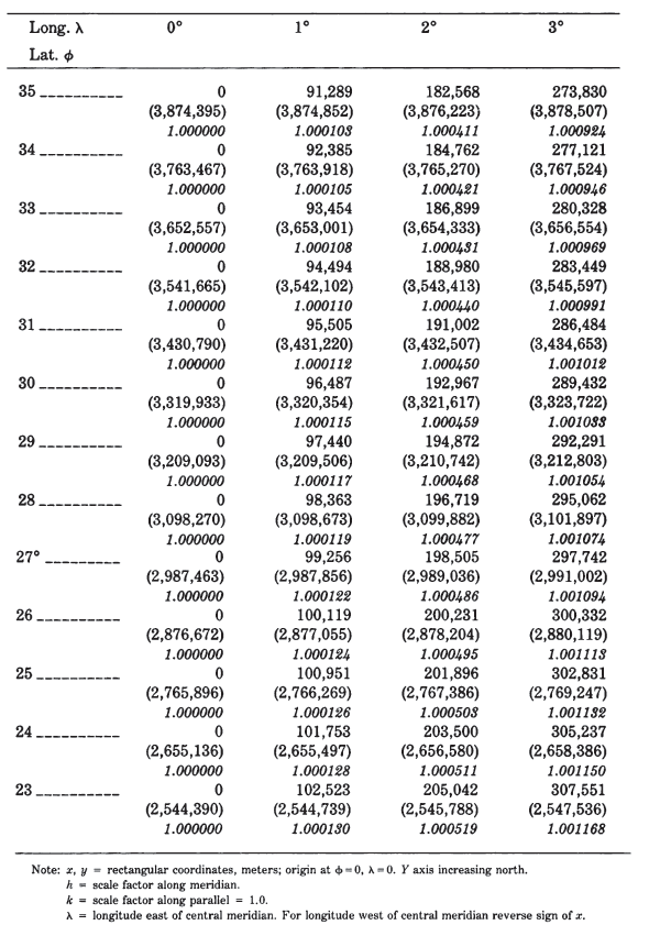
Polar coordinates for the Albers Equal-Area Conic are given for both the spherical and ellipsoidal forms, using standard parallels of lat. 29.5° and 45.5° N. (table 15). A graticule extended to the North Pole is shown in figure 20. TABLE 15.—Albers Equal-Area Conic projection: Polar coordinates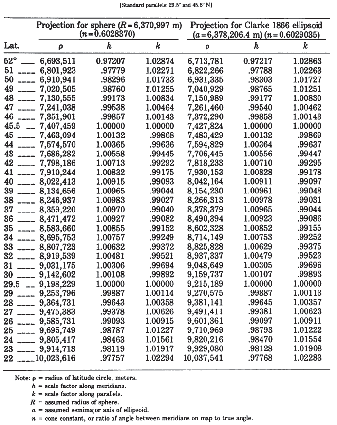
To convert coordinates measured on an existing map, the user may choose any meridian for $\lambda_0$. and therefore for the Y axis, and any latitude for $\phi_0$. The X axis then is placed perpendicular to the Y axis at $\phi_0$.
15. LAMBERT CONFORMAL CONIC PROJECTION #
SUMMARY #
- Conic
- Conformal
- Parallels are unequally spaced arcs of concentric circles, more closely spaced near the center of the map. Meridians are equally spaced radii of the same circles, thereby cutting parallels at right angles.
- Scale is true along two standard parallels, normally, or along just one.
- Pole in same hemisphere as standard parallels is a point; other pole is at infinity.
- Used for maps of countries and regions with predominant east-west expanse.
- Presented by Lambert in 1772.
HISTORY #
The Lambert Conformal Conic projection (fig. 21) was almost completely overlooked between its introduction and its revival by the U.S. Coast and Geodetic Survey (Deetz, 1918b), although France had introduced an approximate version, calling it “Lambert,” for battle maps of the First World War (Mugnier, 1983). It was the first new projection which Johann Heinrich Lambert presented in his Beitrage (Lambert, 1772), the publication which contained his Transverse Mercator described previously. In some atlases, particularly British, the Lambert Conformal Conic is called the “Conical Orthomorphic” projection.
FIGURE 21.—Lambert Conformal Conic projection, with standard parallels 20° and 60° N. North America is illustrated here to show the change in spacing of the parallels. When used for maps of the conterminous United States or individual States, standard parallels are 33° and 45° N.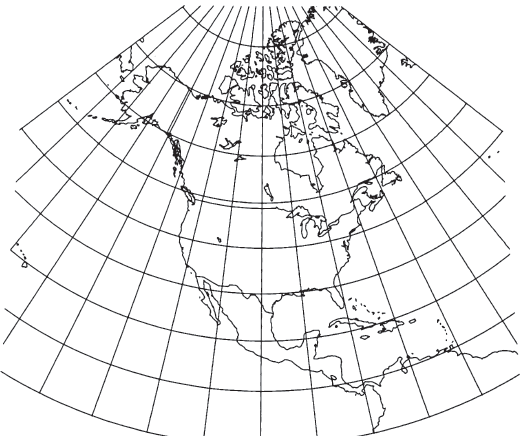
Lambert developed the regular Conformal Conic as the oblique aspect of a family containing the previously known polar Stereographic and regular Mercator projections. As he stated,
Stereographic representations of the spherical surface, as well as Mercator’s nautical charts, have the peculiarity that all angles maintain the sizes that they have on the surface of the globe. This yields the greatest similarity that any plane figure can have with one drawn on the surface of a sphere. The question has not been asked whether this property occurs only in the two methods of representation mentioned or whether these two representations, so different in appearances, can be made to approach each other through intermediate stages. * * * if there are stages intermediate to these two representations, they must be sought by allowing the angle of intersection of the meridians to be arbitrarily larger or smaller than its value on the surface of the sphere. This is the way in which I shall now proceed (Lambert, 1772, p. 28, translation by Tobler).
Lambert then developed the mathematics for both the spherical and ellipsoidal forms for two standard parallels and included a small map of Europe as an example (Lambert, 1772, p. 28-38, 87-89).
FEATURES #
Many of the comments concerning the appearance of the Albers and the selection of its standard parallels apply to the Lambert Conformal Conic when an area the size of the conterminous United States or smaller is considered. As stated before, the spacing of the parallels must be measured to distinguish among the various conic projections for such an area. If the projection is extended toward either pole and the Equator, as on a map of North America, the differences become more obvious. Although meridians are equally spaced radii of the concentric circular arcs representing parallels of latitude, the parallels become further apart as the distance from the central parallels increases. Conformality fails at each pole, as in the case of the regular Mercator. The pole in the same hemisphere as the standard parallels is shown on the Lambert Conformal Conic as a point. The other pole is at infinity. Straight lines between points approximate great circle arcs for maps of moderate coverage, but only the Gnomonic projection rigorously has this feature and then only for the sphere.
Two parallels may be made standard or true to scale, as well as conformal. It is also possible to have just one standard parallel. Since there is no angular distortion at any parallel (except at the poles), it is possible to change the standard parallels to just one, or to another pair, just by changing the scale applied to the existing map and calculating a pair of standard parallels fitting the new scale. This is not true of the Albers, on which only the original standard parallels are free from angular distortion.
If the standard parallels are symmetrical about the Equator, the regular Mercator results (although formulas must be revised). If the only standard parallel is a pole, the polar Stereographic results.
The scale is too small between the standard parallels and too large beyond them. This applies to the scale along meridians, as well as along parallels, or in any other direction, since they are equal at any given point. Thus, in the State Plane Coordinate Systems (SPCS) for States using the Lambert, the choice of standard parallels has the effect of reducing the scale of the central parallel by an amount which cannot be expressed simply in exact form, while the scale for the central meridian of a map using the Transverse Mercator is normally reduced by a simple fraction. The scale is constant along any given parallel. While it equals the nominal scale at the standard parallels, it actually changes most slowly in a north-south direction at a parallel nearly halfway between the two standard parallels.
USAGE #
It was only a couple of decades after the Coast and Geodetic Survey began publishing tables for the Lambert Conformal Conic projection (Deetz, 1918a 1918b) that the projection was adopted officially for the SPCS for States of predominantly east-west expanse. The prototype was the North Carolina Coordinate System, established in 1933. Within a year or so, similar systems were devised for many other States, while a Transverse Mercator system was prepared for the remaining States. One or more zones is involved in the system for each State (see table 8) (Mitchell and Simmons, 1945, p. vi). In addition, the Lambert is used for the Aleutian Islands of Alaska, Long Island in New York, and northwestern Florida, although the Transverse Mercator (and Oblique Mercator in one case) is used for the rest of each of these States.
The Lambert Conformal Conic is used for the 1:1,000,000-scale regional world aeronautical charts, the 1:500,000-scale sectional aeronautical charts, and 1:500,000-scale State base maps (all 48 contiguous States1 have the same standard parallels of lat. 33° and 45° N., and thus match). Also cast on the Lambert are most of the 1:24,000-scale 7½-minute quadrangles prepared after 1957 which lie in zones for which the Lambert is the base for the SPCS. In the latter case, the standard parallels for the zone are used, rather than parameters designed for the individual quadrangles. Thus, all quadrangles for a given zone may be mosaicked exactly. (The projection used previously was the Polyconic, and some recent quadrangles are being produced to the Universal Transverse Mercator projection.)
The Lambert Conformal Conic has also been adopted as the official topographic projection for some other countries. It appears in The National Atlas (USGS, 1970, p. 116) for a map of hurricane patterns in the North Atlantic, and the Lambert is used by the USGS for a map of the United States showing all 50 States in their true relative positions. The latter map is at scales of both 1:6,000,000 and 1:10,000,000, with standard parallels 37° and 65° N.
In 1962, the projection for the International Map of the World at a scale of 1:1,000,000 was changed from a modified Polyconic to the Lambert Conformal Conic between lats. 84° N. and 80° S. The polar Stereographic projection is used in the remaining areas. The sheets are generally 6° of longitude wide by 4° of latitude high. The standard parallels are placed at one-sixth and five-sixths of the latitude spacing for each zone of 4° latitude, and the reference ellipsoid is the International (United Nations, 1963, p. 9-27). This specification has been subsequently used by the USGS in constructing several maps for the IMW series.
Perhaps the most recent new topographic use for the Lambert Conformal Conic projection by the USGS is for middle latitudes of the 1:1,000,000-scale geologic series of the Moon and for some of the maps of Mercury, Mars, and Jupiter’s satellites (see table 6).
FORMULAS FOR THE SPHERE #
For the projection as normally used, with two standard parallels, the equations for the sphere may be written as follows: given $R, \phi_1, \phi_2, \phi_0, \lambda_0, \phi$, and $\lambda$ (see numerical examples):
$\phi_1,\phi_2=$ standard parallels.
The Y axis lies along the central meridian $\lambda_0$, $y$ increasing northerly; the X axis intersects perpendicularly at $\phi_0, x$ increasing easterly. If $(\lambda-\lambda_0)$ exceeds the range $\pm180°$, 360° should be added or subtracted. Constants $n, F$, and $\rho_0$ need to be determined only once for the entire map.
If only one standard parallel is desired, equation (15-3) is indeterminate, but $n=\sin\phi_1$. The scale along meridians or parallels, using equations (4-4) or (4-5),
For the inverse formulas for the sphere, given $R,\phi_1,\phi_2,\phi_0,\lambda_0, x$ and $y$: $n, F,$ and $\rho_0$ are calculated from equations (15-3), (15-2), and (15-1a), respectively.Then,
The standard parallels normally used for maps of the conterminous United States are lats. 33° and 45° N., which give approximately the least overall error within those boundaries. The ellipsoidal form is used for such maps, based on the Clarke 1866 ellipsoid (Adams, 1918).
The standard parallels of 33° and 45° were selected by the USGS because of the existing tables by Adams (1918), but Adams chose them to provide a maximum scale error between latitudes 30.5° and 47.5° of one-half of 1 percent. A maximum scale error of 2.5 percent occurs in southernmost Florida (Deetz and Adams, 1934, p. 80). Other standard parallels would reduce the maximum scale error for the United States, but at the expense of accuracy in the center of the map.
FORMULAS FOR THE ELLIPSOID #
The ellipsoidal formulas are essential when applying the Lambert Conformal Conic to mapping at a scale of 1:100,000 or larger and important at scales of 1:5,000,000. Given $a, e, \phi_1, \phi_2, \phi_0, \lambda_0, \phi$, and $\lambda$ (see numerical examples):
When the above equations for the ellipsoidal form are used, they give values of $n$ and $\rho$ slightly different from those in the accepted tables of coordinates for a map of the United States, according to the Lambert Conformal Conic projection. The discrepancy is 35-50 m in the radius and 0.0000035 in $n$. The rectangular coordinates are correspondingly affected. The discrepancy is less significant when it is realized that the radius is measured to the pole, and that the distance from the 50th parallel to the 25th parallel on the map at full scale is only 12 m out of 2,800,000 or 0.0004 percent. For calculating convenience 60 years ago, the tables were, in effect, calculated using instead of equation (15-9),
For the existing tables, then, $\phi_g$, the geocentric latitude, was used for convenience in place of $\chi$ , the conformal latitude (Adams, 1918, p. 6-9, 34). A comparison of series equations (3-3) and (3-30), or of the corresponding columns in table 3, shows that the two auxiliary latitudes $\chi$ and $\phi_g$ are numerically very nearly the same.
There may be much smaller discrepancies found between coordinates as calculated on modern computers and those listed in tables for the SPCS. This is due to the slightly reduced (but sufficient) accuracy of the desk calculators of 30-40 years ago and the adaptation of formulas to be more easily utilized by them. To obtain SPCS coordinates, the appropriate “false easting” is added to $x$ after calculation using (14-1).
The inverse formulas for ellipsoidal coordinates, given $a, e, \phi_1, \phi_2, \phi_0, \lambda_0, x$, and $y$: $n, F$, and $\rho_0$ are calculated from equations (15-8), (15-10), (15-7a), respectively . Then
Equation (7-9) involves rapidly converging iteration: Calculate t from (15-11). Then, assuming an initial trial $\phi$ equal to $(\pi/2−2\arctan t)$ in the right side of equation (7—9) , calculate $\phi$ on the left side. Substitute the calculated $\phi$ into the right side, calculate a new $\phi$, etc., until $\phi$ does not change significantly from the preceding trial value of $\phi$.
To avoid iteration, series (3-5) may be used with (7-13) in place of (7-9).
If rectangular coordinates for maps based on tables using geocentric latitude are to be converted to latitude and longitude, the inverse formulas are the same as those above except that equation (15-9b) is used instead of (15-9) for calculations leading to $n, F$, and $\rho_0$, and equation (7-9) or (3-5) and (7-13), is replaced with the following which does not involve iteration:
Polar coordinates for the Lambert Conformal Conic are given for both the spherical and ellipsoidal forms using standard parallels of 33° and 45° N, (table 16). The data based on geocentric latitude are given for comparison. A graticule extending to the North Pole is shown in figure 21. TABLE 16.—Lambert Conformal Conic projection: Polar coordinates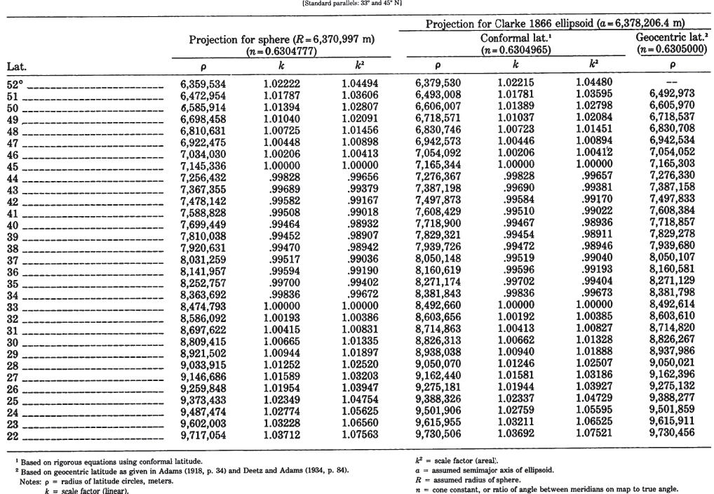
To convert from tabular rectangular coordinates to $\phi$ and $\lambda$, it is necessary to subtract any “false easting” from $x$ and “false northing” from $y$ before inserting $x$ and $y$ into the inverse formulas. To convert coordinates measured on an existing Lambert Conformal Conic map (or other regular conic projection), the user may choose any meridian for $\lambda_0$ and therefore for the Y axis , and any latitude for $\phi_0$. The X axis then is placed perpendicular to the Y axis at $\phi_0$.
16. EQUIDISTANT CONIC PROJECTION #
SUMMARY #
- Conic.
- Equidistant.
- Parallels, including poles, are arcs of concentric circles, equally spaced for the sphere, at true spacing for the ellipsoid.
- Meridians are equally spaced radii of the same circles, thereby cutting parallels at right angles.
- Scale is true along all meridians and along one or two standard parallels.
- Used for maps of small countries and regions and of larger areas with predominant east-west expanse.
- Rudimentary form developed by Claudius Ptolemy about A.D. 150
HISTORY #
The simplest kind of conic projection is the Equidistant Conic, often called Simple Conic, or just Conic projection. It is the projection most likely to be found in atlases for maps of small countries, with its equally spaced straight meridians and equally spaced circular parallels. A rudimentary version was described by the astronomer and geographer Claudius Ptolemy about A.D. 150. Probably born in Greece about A.D. 90, he spent most of his life in or near Alexandria, Egypt, and died about A.D. 168. His greatest works were the Almagest, describing his scientific theories, and the Geographia, which dwelt on mapmaking. These were revived in the 15th century as the most authoritative existing standards.
In developing this projection, Ptolemy did not discuss cones, and a cone would not properly fit his specifications, but he said (Geographia, Book 1, ch. 20):
When we cast a glance upon the middle of the northern quarter of the globe in which the greatest part of the oikumene [or ecumene, or inhabited world] lies, then the meridians give the impression of being straight lines if we turn the globe thus that the meridians successively come out of their sideward situation right before the spectator, so that the eye comes in their plane. The parallels give clearly the impression of arcs of circles which turn their convex side to the south (Keuning, 1955, p. 9).
Ptolemy’s conic projection extends from latitudes approximating 63°N. to 16°S. Although meridians north of the Equator fan out as straight radii from the center of the circular parallels, they break at the Equator to connect with straight lines to points along the southernmost parallel which are the same distance apart as corresponding points at 16°N.
Johannes Ruysch (?-1533) modified this approach to continue meridians as straight radii below the Equator in a world map of 1508, and Gerardus Mercator made other modifications in the mid-16th century. The Equidistant Conic with two standard parallels is credited to Joseph Nicolas De l’Isle (1688- 1768), of an illustrious French mapmaking family. He used it for a map of Russia in 1745. There were differences in his approach, however, which resulted in meridians which are not radii of the circular arcs representing the circles.
Several Scot (Murdoch), Swiss (Euler), English (Everett), and Russian (Vitkovskiy, Kavrayskiy, and others) mathematicians published papers between 1758 and 1934 describing means of selecting the two standard parallels so that distortion is minimized using various criteria. Each of them used the same basic conic projection with concentric circular parallels and straight meridians for radii (Snyder, 1978a). The name of one of them, V. V. Kavrayskiy (or Kavraisky), has been mistakenly applied in some U.S. literature to the basic projection, but his contribution did not occur until 1934.
The Equidistant Conic projection (fig. 22) is neither conformal (like the Lambert Conformal Conic) nor equal-area (like the Albers), but it serves as a compromise between them. The Lambert parallels are more widely spaced away from the central parallel, and the Albers parallels become closer together. The parallels on the Equidistant Conic remain equally spaced on the spherical version (as they are on the sphere) and nearly so on the ellipsoidal version (with the same spacing as the distances along the meridians on the ellipsoid).
As on other normal conics, the meridians are equally spaced radii of the concentric circular arcs which form the parallels. The meridians are spaced at equal angles which are less than the true angles between the meridians; the ratio is called the cone constant, as it is on other conic projections. The poles are normally also plotted as circular arcs.
Either one or two parallels may be made standard or true to scale. There is no shape, area, or scale distortion along the standard parallels. While meridians are at correct scale everywhere, the scale along the parallels between the standard parallels (if there are two) is too small, and the scale along parallels beyond the standard parallel(s) is too great.
If the one standard parallel is the Equator, the Equidistant Conic projection becomes the Plate Carrée form of the Equidistant Cylindrical, but the formulas must be changed. If the two standard parallels are symmetrical about the Equator, the Equirectangular results. If the standard parallel is the pole, the Azimuthal Equidistant projection is obtained. FIGURE 22.—Equidistant Conic projection, with standard parallels 20° and 60° N. All of North America is included to show that parallels remain equidistant. Compare figures 20 and 21.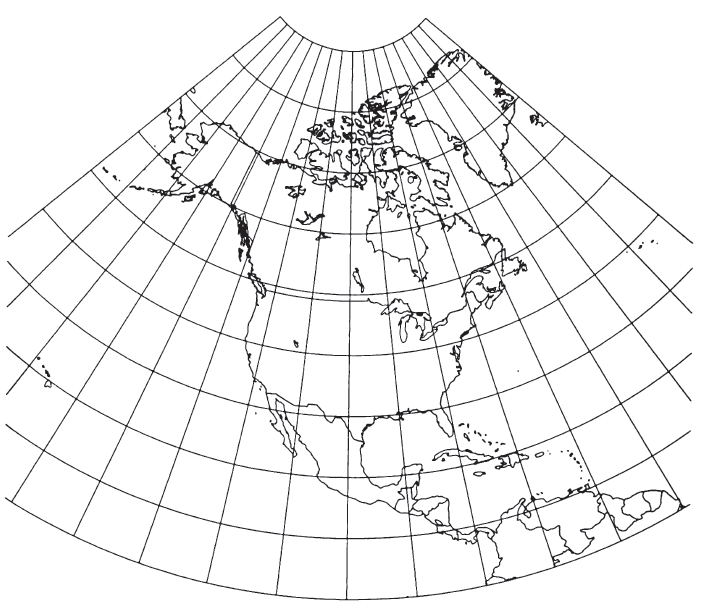
USAGE #
The Equidistant Conic projection is commonly used in the spherical form in atlases for maps of small countries. Its only use by the USGS has been in an approximate ellipsoidal form for Alaska Maps “B” and “E,” but the projection name applied is “Modified Transverse Mercator” (see p. 63), due to the original manner of construction. The formulas for the ellipsoidal version were apparently first published in Snyder (1978a), although there may be several de facto usages of the ellipsoidal form such as the above. For example, the New Mexico Planning Survey in effect devised such a projection in 1936 for the mapping of that State, calling it a “Modified Conic Projection” (Thomas E. Henderson, pers. comm., 1985).
FORMULAS FOR THE SPHERE #
For the Equidistant Conic projection with two standard parallels, given $R, \phi1, \phi2, \phi_0, \lambda_0, \phi,$ and $\lambda$, to find $x$ and $y$ (see numerical examples):
$\phi_0, \lambda_0 =$ the latitude and longitude, for the origin of the rectangular coordinates.
$\phi_1,\phi_2=$ standard parallels.
The Y axis lies along the central meridian $\lambda_0$, $y$ increasing northerly. The X axis intersects perpendicularly at $\phi_0$, $x$ increasing easterly. If $(\lambda - \lambda_0)$ exceeds the range $\pm180°$, 360° should be added or subtracted to place it within the range. Constants $n, G$, and $\rho_0$ need to be determined only once for the entire map.
If only one standard parallel $\phi_1$, is desired, equation (16-4) is indeterminate, but $n = \sin\phi_1$. The scale $h$ along meridians is 1.0. Along parallels, using equation (4-5), the scale is
The maximum angular deformation may be calculated from equation (4-9). As on other regular conics, distortion is only a function of latitude.
For the inverse formulas for the sphere, given $R, \phi1, \phi2, \phi_0, \lambda_0, x,$ and $y$ to find $\phi$ and $\lambda$: $n, G$, and $\rho_0$ are calculated from equations (16-4), (16-3), and (16-2), respectively. Then,
FORMULAS FOR THE ELLIPSOID #
For mapping of regions smaller than the United States at scales greater than 1:5,000,000, using the Equidistant Conic projection, the ellipsoidal formulas should be considered. Given $a, e, \phi_1, \phi_2, \phi_0, \lambda_0, \phi$ and $\lambda$, to find $x$ and $y$ (see numerical examples):
with the same subscripts 1,2, or none applied to $m$ and $\phi$ in equation (14-15), and 0, 1, 2, or none applied to $M$ and $\phi$ in equation (3-21). For improved computational efficiency using the series, see p. 19. As with other conics, a negative $n$ and $\rho$ result for projections centered in the Southern Hemisphere. If $\phi_1 = \phi_2$ for the Equidistant Conic with a single standard parallel, equation (16-10) is indeterminate, but $n = \sin\phi_1$. Origin and orientation of axes for x and y are the same as those for the spherical form. Constants $n, G,$ and $\rho_0$ may be determined just once for the entire map.
For the inverse formulas for the ellipsoid, given $a, e, \phi_1, \phi_2, \phi_0, \lambda_0, x,$ and $y$, to find $\phi$ and $\lambda$: $n, G,$ and $\rho_0$ are calculated from equations (16-10), (16-11), and (16-9), respectively. Then
Polar coordinates for the Equidistant Conic projection for a map of the United States, assuming standard parallels of lat. 29.5° and 45.5°N., are listed in table 17 for both the spherical and ellipsoidal forms. A graticule extended to the North Pole is shown in figure 22. TABLE 17.— Equidistant Conic projection: Polar coordinates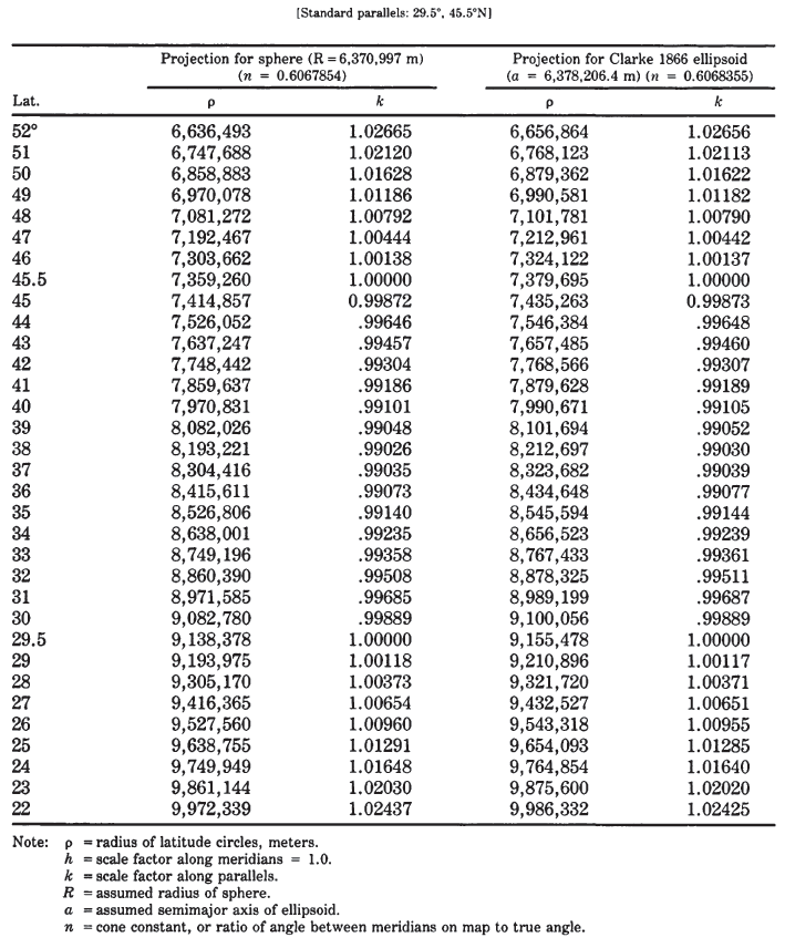
17. BIPOLAR OBLIQUE CONIC CONFORMAL PROJECTION #
SUMMARY #
- Two oblique conic projections, side-by-side, but with poles 104° apart.
- Conformal.
- Meridians parallels are complex curves, intersecting at right angles.
- Scale is true along two standard transformed parallels on each conic projection, neither of these lines following any geographical meridian or parallel.
- Very small deviation from conformality, where the two conic projections join.
- Specially developed for a map of the Americas. Used only in spherical form.
- Presented by Miller and Briesemeister in 1941.
HISTORY #
A “tailor-made” projection is one designed for a certain geographical area. O. M. Miller used the term for some projections which he developed for the American Geographical Society (AGS) or for their clients. The Bipolar Oblique Conic Conformal projection, developed with William A. Briesemeister, was presented in 1941 and designed specifically for a map of North and South America constructed in several sheets by the AGS at a scale of 1:5,000,000 (Miller, 1941).
It is an adaptation of the Lambert Conformal Conic projection to minimize scale error over the two continents by accommodating the fact that North America tends to curve toward the east as one proceeds from north to south, while South America tends to curve in the opposite direction. Because of the relatively small scale of the map, the Earth was treated as a sphere. To construct the map, a great circle arc 104° long was selected to cut through Central America from southwest to northeast, beginning at lat. 20° S. and long. 110° W. and terminating at lat. 45°N. and the resulting longitude of about 19°59'36" W.
The former point is used as the pole and as the center of transformed parallels of latitude for an Oblique Conformal Conic projection with two standard parallels (at polar distances of 31° and 73°) for all the land in the Americas southeast of the 104° great circle arc. The latter point serves as the pole and center of parallels for an identical projection for all land northwest of the same arc. The inner and outer standard parallels of the northwest portion of the map, thus, are tangent to the outer and inner standard parallels, respectively, of the southeast portion, touching at the dividing line (104°-31° = 73°).
The scale of the map was then increased by about 3.5 percent, so that the linear scale error along the central parallels (at a polar distance of 52°, halfway between 31° and 73°) is equal and opposite in sign (-3.5 percent) to the scale error along the two standard parallels (now +3.5 percent) which are at the normal map limits. Under these conditions, transformed parallels at polar distances of about 36.34° and 66.58° are true to scale and are actually the standard transformed parallels.
The use of the Oblique Conformal Conic projection was not original with Miller and Briesemeister. The concept involves the shifting of the graticule of meridians and parallels for the regular Lambert Conformal Conic so that the pole of the projection is no longer at the pole of the Earth. This is the same principle as the transformation for the Oblique Mercator projection. The bipolar concept is unique, however, and it has apparently not been used for any other maps.
FIGURE 23.— Bipolar Oblique Conic Conformal projection used for various geologic maps. The American Geographical Society, under O. M. Miller, prepared the base map used by the USGS. (Prepared by Tau Rho Alpha.)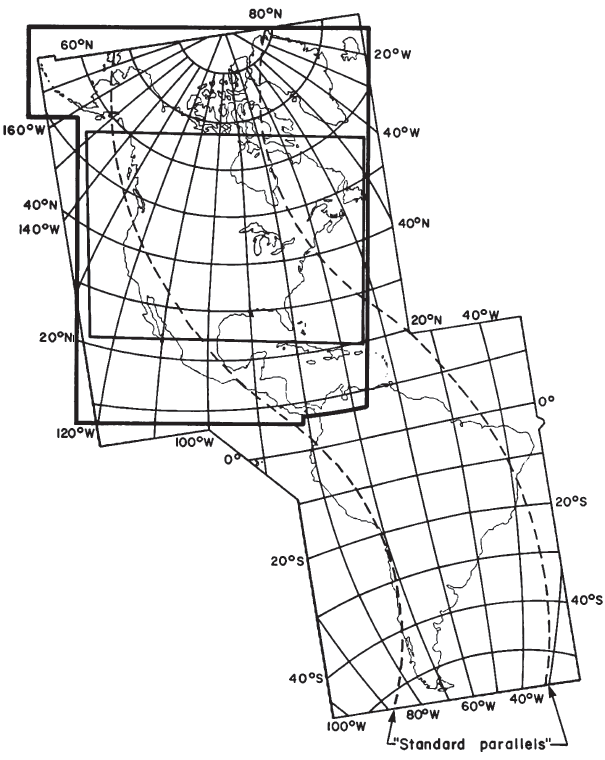
FEATURES AND USAGE #
The Geological Survey has used the North American portion of the map for the Geologic Map (1965), the Basement Map (1967), the Geothermal Map, and the Metallogenic Map, all retaining the original scale of 1:5,000,000. The Tectonic Map of North America (1969) is generally based on the Bipolar Oblique Conic Conformal, but there are modifications near the edges. An oblique conic projection about a single transformed pole would suffice for either one of the continents alone, but the AGS map served as an available base map at an appropriate scale. In 1979, the USGS decided to replace this projection with the Transverse Mercator for a map of North America.
The projection is conformal, and each of the two conic projections has all the characteristics of the Lambert Conformal Conic projection, except for the important difference in location of the pole, and a very narrow band near the center. While meridians and parallels on the oblique projection intersect at right angles because the map is conformal, the parallels are not arcs of circles, and the meridians are not straight, except for the peripheral meridian from each transformed pole to the nearest normal pole.
The ‘scale is constant along each circular arc centered on the transformed pole for the conic projection of the particular portion of the map. Thus, the two lines at a scale factor of 1.035, that is, both pairs of the official standard transformed parallels, are mapped as circular arcs forming the letter “S.” The 104° great circle arc separating the two oblique conic projections is a straight line on the map, and all other straight lines radiating from the poles for the respective conic projections are transformed meridians and are therefore great circle routes. These straight lines are not normally shown on the finished map.
At the juncture of the two conic projections, along the 104" axis, there is actually a slight mathematical discontinuity at every point except for the two points at which the transformed parallels of polar distance 31° and 73° meet. If the conic projections are strictly followed, there is a maximum discrepancy of 1.6 mm at the 1:5,000,000 scale at the midpoint of this axis, halfway between the poles or between the intersections of the axis with the 31° and 73° transformed parallels. In other words, a meridian approaching the axis from the south is shifted up to 1.6 mm along the axis as it crosses. Along the axis, but beyond the portion between the lines of true scale, the discrepancy increases markedly, until it is over 240 mm at the transformed poles. These latter areas are beyond the needed range of the map and are not shown, just as the polar areas of the regular Lambert Conformal Conic are normally omitted. This would not happen if the Oblique Equidistant Conic projection were used.
The discontinuity was resolved by connecting the two arcs with a straight line tangent to both, a convenience which leaves the small intermediate area slightly nonconformal. This adjustment is included in the formulas below.
FORMULAS FOR THE SPHERE #
The original map was prepared by the American Geographical Society, in an era when automatic plotters and easy computation of coordinates were not yet present. Map coordinates were determined by converting the geographical coordinates of a given graticule intersection to the transformed latitude and longitude based on the poles of the projection, then to polar coordinates according to the conformal projection, and finally to rectangular coordinates relative to the selected origin.
The following formulas combine these steps in a form which may be programmed for the computer. First, various constants are calculated from the above parameters, applying to the entire map. Since only one map is involved, the numerical values are inserted in formulas, except where the numbers are transcendental and are referred to by symbols.
If the southwest pole is at point A, the northeast pole is at point B, and the center point on the axis is C,
If $Az_B$, is greater than $Az_{BA}$ (from equation (17-7)), go to equation (17-23). Otherwise proceed to equation (17-16) for the projection from pole $B$.
For the inverse formulas for the Bipolar Oblique Conic Conformal, the constants for the map must first be calculated from equations (17-1)- (17-13). Given x and y coordinates based on the above axes, they are then converted to the skew coordinates:
A table of rectangular coordinates is given in table 18, based on a radius R of 1.0, while a graticule is shown in figure 23. TABLE 18.— Bipolar Oblique Conic Conformal Projection: Rectangular coordinates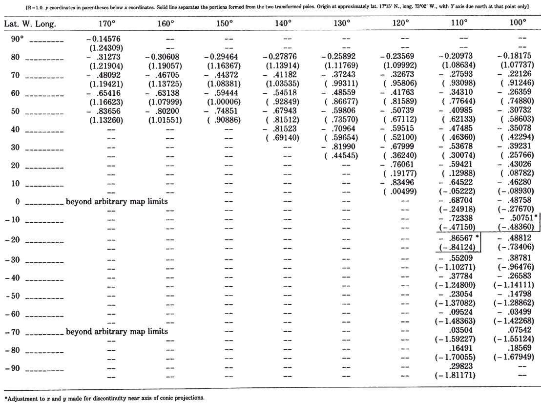
18. POLYCONIC PROJECTION #
SUMMARY #
- Neither conformal nor equal-area.
- Parallels of latitude (except for Equator) are arcs of circles, but are not concentric.
- Central meridian and Equator are straight lines; all other meridians are complex curves.
- Scale is true along each parallel and along the central meridian, but no parallel is “standard.”
- Free of distortion only along the central meridian.
- Used almost exclusively in slightly modified form for large-scale mapping in the United States until the 1950’s.
- Was apparently originated about 1820 by Hassler.
HISTORY #
Shortly before 1820, Ferdinand Rudolph Hassler (fig. 24) began to promote the Polyconic projection, which was to become a standard for much of the official mapping of the United States (Deetz and Adams, 1934, p. 58-60). FIGURE 24.— Ferdinand Rudolph Hassler (1770-1843), first Superintendent of the U.S. Coast Survey and presumed inventor of the Polyconic projection. As a result of his promotion of its use, it became the projection exclusively used for USGS topographic quadrangles for about 70 years.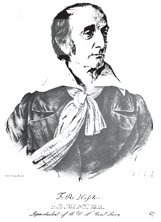
Born in Switzerland in 1770, Hassler arrived in the United States in 1805 and was hired 2 years later as the first head of the Survey of the Coast. He was forced to wait until 1811 for funds and equipment, meanwhile teaching to maintain income. After funds were granted, he spent 4 years in Europe securing equipment. Surveying began in 1816, but Congress, dissatisfied with the progress, took the Survey from his control in 1818. The work only foundered. It was returned to Hassler, now superintendent, in 1832. Hassler died in Philadelphia in 1843 as a result of exposure after a fall, trying to save his instruments in a severe wind and hailstorm, but he had firmly established what later became the U.S. Coast and Geodetic Survey (Wraight and Roberts, 1957) and is now the National Ocean Service.
The Polyconic projection, usually called the American Polyconic in Europe, achieved its name because the curvature of the circular arc for each parallel on the map is the same as it would be following the unrolling of a cone which had been wrapped around the globe tangent to the particular parallel of latitude, with the parallel traced onto the cone. Thus, there are many (“poly-”) cones involved, rather than the single cone of each regular conic projection. As Hassler himself described the principles, “[t]his distribution of the projection, in an assemblage of sections of surfaces of successive cones, tangents to or cutting a regular succession of parallels, and upon regularly changing central meridians, appeared to me the only one applicable to the coast of the United States” (Hassler, 1825, p. 407-408).
The term “polyconic” is also applied generically by some writers to other projections on which parallels are shown as circular arcs. Most commonly, the term applies to the specific projection described here. FIGURE 25.— North America on a Polyconic projection grid, central meridian long. 100° W., using a 10° interval. The parallels are arcs of circles which are not concentric, but have radii equal to the radius of curvature of the parallel at the Earth’s surface. The meridians are complex curves formed by connecting points marked off along the parallels at their true distances. Used by the USGS for topographic quadrangle maps.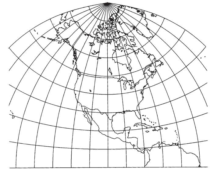
FEATURES #
The Polyconic projection (fig. 25) is neither equal-area nor conformal. Along the central meridian, however, it is both distortion free and true to scale. Each parallel is true to scale, but the meridians are lengthened by various amounts to cross each parallel at the correct position along the parallel, so that no parallel is standard in the sense of having conformality (or correct angles), except at the central meridian. Near the central meridian, which is the case with 7½-minute quadrangles, distortion is extremely small. The Polyconic projection is universal in that tables of rectangular coordinates may be used for any Polyconic projection of the same ellipsoid by merely applying the proper scale and central meridian. U.S. Coast and Geodetic Survey Special Publication No. 5 (1900) replaced tables published in 1884 and was often reprinted because of the universality of the projection (the Clarke 1866 is the reference ellipsoid). Polyconic quadrangle maps prepared to the same scale and for the same central meridian and ellipsoid will fit exactly from north to south. Since they are drawn in practice with straight meridians, they also fit east to west, but discrepancies will accumulate if mosaicking is attempted in both directions.
The parallels are all circular arcs, with the centers of the arcs lying along an extension of the straight central meridian, but these arcs are not concentric. Instead, as noted earlier, the radius of each arc is that of the circle developed from a cone tangent to the sphere or ellipsoid at the latitude. For the sphere, each parallel has a radius proportional to the cotangent of the latitude. For the ellipsoid, the radius is slightly different. The Equator is a straight line in either case. Along the central meridian, the parallels are spaced at their true intervals. For the sphere, they are therefore equidistant. Each parallel is marked off for meridians equidistantly and true to scale. The points so marked are connected by the curved meridians.
USAGE #
As geodetic and coastal surveying began in earnest during the 19th century, the Polyconic projection became a standard, especially for quadrangles. Most coastal charts produced by the Coast Survey and its successor during the 19th century were based on one or more variations of the Polyconic projection (Shalowitz, 1964, p. 138-141). The name of the projection appears on a later reprint of one of the first published USGS topographic quadrangles, which appeared in 1886. In 1904, the USGS published tables of rectangular coordinates extracted from an 1884 Coast and Geodetic Survey report. They were called “coordinates of curvature,” but were actually coordinates for the Polyconic projection, although the latter term was not used (Gannett, 1904, p. 37-48).
As a 1928 USGS bulletin of topographic instructions stated (Beaman, 1928, p. 163):
The topographic engineer needs a projection which is simple in construction, which can be used to represent small areas on any part of the globe, and which, for each small area to which it is applied, preserves shapes, areas, distances, and azimuths in their true relation to the surface of the earth. The polyconic projection meets all these needs and was adopted for the standard topographic map of the United States, in which the 1° quadrangle is the largest unit *** and the 15’ quadrangle is the average unit. *** Misuse of this projection in attempts to spread it over large areas – that is, to construct a single map of a large area-has developed serious errors and gross exaggeration of details. For example, the polyconic projection is not at all suitable for a single-sheet map of the United States or of a large State, although it has been so employed.
When coordinate plotters and published tables for the State Plane Coordinate System (SPCS) became available in the late 1950’s, the USGS ceased using the Polyconic for new maps, in favor of the Transverse Mercator or Lambert Conformal Conic projections used with the SPCS for the area involved. Some of the quadrangles prepared on one or the other of these projections have continued to carry the Polyconic designation, however.
The Polyconic projection was also used for the Progressive Military Grid for military mapping of the United States. There were seven zones, A-G, with central meridians every 8° west from long. 73° W. (zone A), each zone having an origin at lat. 40°30’ N. on the central meridian with coordinates $x= 1,000,000$ yards, $y =2,000,000$ yards (Deetz and Adams, 1934, p. 87-90). Some USGS quadrangles of the 1930’s and 1940’s display tick marks according to this grid in yards, and many quadrangles then prepared by the Army Map Service and sold by the USGS show a complete grid pattern. This grid was incorporated intact into the World Polyconic Grid (WPG) until both were superseded by the Universal Transverse Mercator grid (Mugnier, 1983).
While quadrangles based on the Polyconic provide low-distortion mapping of the local areas, the inability to mosaic these quadrangles in all directions without gaps makes them less satisfactory for a larger region. Quadrangles based on the SPCS may be mosaicked over an entire zone, at the expense of increased distortion.
For an individual quadrangle 7½ or 15 minutes of latitude or longitude on a side, the distance of the quadrangle from the central meridian of a Transverse Mercator zone or from the standard parallels of a Lambert Conformal Conic zone of the SPCS has much more effect than the type of projection upon the variation in measurement of distances on quadrangles based on the various projections. If the central meridians or standard parallels of the SPCS zones fall on the quadrangle, a change of projection from Polyconic to Transverse Mercator or Lambert Conformal Conic results in a difference of less than 0.001 mm in the measurement of the 700-800 mm diagonals of a 7½-minute quadrangle. If the quadrangle is near the edge of a zone, the discrepancy between measurements of diagonals on two maps of the same quadrangle, one using the Transverse Mercator or Lambert Conformal Conic projection and the other using the Polyconic, can reach about 0.05 mm. These differences are exceeded by variations in expansion and contraction of paper maps, so that these mathematical discrepancies apply only to comparisons of stable-base maps.
Actually, the central meridian of a 7½-minute Polyconic quadrangle may lie along the edge of the map, since 15-minute quadrangles were frequently cut and enlarged to achieve the less extensive coverage. This has a negligible effect upon the map geometry.
Before the Lambert became the projection for the 1:500,000 State base map series, a modified form of the Polyconic was used, but the details are unclear. The Polyconic was used for the base maps of Alaska until 1972. It has also been used for maps of the United States; but, as stated above, the distortion is excessive at the east and west coasts, and most current maps are drawn to either the Lambert or Albers Conic projections. There are several other modified Polyconic projections, in use or devised, including the Rectangular Polyconic and Bousfield’s modification used for northern Canada (Haines, 1981). The best known is that used for the International Map of the World, described on p. 131.
GEOMETRIC CONSTRUCTION #
Because of the simplicity of construction using universal tables with which the central meridian and each parallel may be marked off at true distances, the Polyconic projection was favored long after theoretically better projections became known in geodetic circles.
The Polyconic projection must be constructed with curved meridians and parallels if it is used for single-sheet maps of areas with east-west extent of several degrees. Then, however, the inherent distortion is excessive, and a different projection should be considered. For accurate topographic work, the coverage must remain so small that the meridians and parallels may ironically but satisfactorily be drawn as straight-line segments. Official USGS instructions of 1928 declared that
in actual practice on projections of small quadrangles, the parallels are not drawn as arcs of circles, but their intersections with the meridians are plotted from the computed x and y values, and the sections of the parallels between adjacent meridians are drawn as straight lines. In polyconic projections of quadrangles of 1° or smaller meridians may be drawn as straight lines, and in large-scale projections of small quadrangles in low latitudes both meridians and parallels may be drawn as straight lines. For example, the curvature of the parallels of a projection of a 15’ quadrangle on a scale of 1:48,000 in latitudes from 0° to 30° is so small that it can not be plotted, and for a 7½ quadrangle on a scale of 1:31,680 or larger the curvature can not be plotted at any latitude (Beaman, 1928, p. 167).
This instruction is essentially repeated in the 1964 edition (USGS, 1964, p. 12-13). The formulas given below are based on curved meridians.
FORMULAS FOR THE SPHERE #
The principles stated above lead to the following forward formulas for rectangular coordinates for the spherical form of the Polyconic projection, using radians (see numerical examples):
The inverse formulas for the sphere are given here in the form of a Newton-Raphson approximation, which converges to any desired accuracy after several iterations, except that if $|\lambda - \lambda_0|>90°$, a rarely used range, this iteration does not converge, and if $y = -R\phi_0$, it is indeterminate. In the latter case, however,
FORMULAS FOR THE ELLIPSOID #
The forward formulas for the ellipsoidal form of the Polyconic projection are only a little more complicated than those for the sphere. These formulas are theoretically exact. They are adapted from formulas given by the Coast and Geodetic Survey (1946, p. 4) (see numerical examples): If $\phi$ is 0,
If $\phi$ is zero,
As with the inverse spherical formulas, the inverse ellipsoidal formulas are given in a Newton-Raphson form, converging to any desired degree of accuracy after several iterations. As before, if $|\lambda-\lambda_0|>90^\circ$, this iteration does not converge, but the projection should not be used in that range in any case. The formulas may be calculated in the following order, given $a, e, \phi_0, \lambda_0, x,$ and $y$. First $M_0$ is calculated from equation (3-21) above, as in the forward case, with $\phi_0$ for $\phi$ and $M_0$ for $M$.
If $y=M_0$, the iteration is not applicable, but
Table 19 lists rectangular coordinates for a band 3° on either side of the central meridian for the ellipsoid extending from lat. 23° to 50° N. Figure 25 shows the
graticule applied to a map of North America. TABLE 19.— Polyconic Projection: Rectangular coordinates for the Clarke 1866 ellipsoid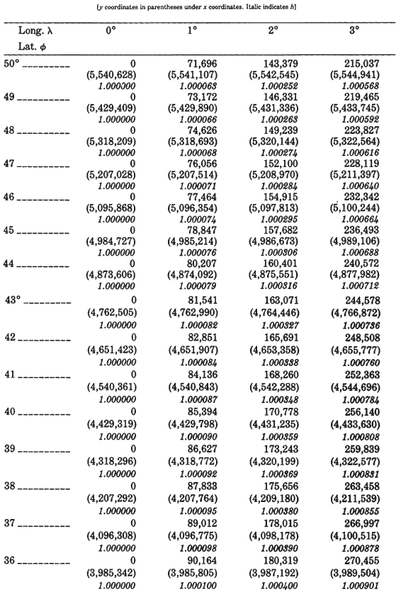
MODIFIED POLYCONIC FOR THE INTERNATIONAL MAP OF THE WORLD #
A modified Polyconic projection was devised by Lallemand of France and in 1909 adopted by the International Map Committee (IMC) in London as the basis for the 1:1,000,000-scale International Map of the World (IMW) series. Used for sheets 6° of longitude by 4° of latitude between lats. 60° N. and 60° S., 12° of longitude by 4° of latitude between lats. 60° and 76° N. or S., and 24° by 4° between lats. 76° and 84° N. or S., the projection differs from the ordinary Polyconic in two principal features: All meridians are straight, and there are two meridians (2° east and west of the central meridian on sheets between lats. 60° N. & S.) that are made true to scale. Between lats. 60° & 76° N. and S., the meridians 4° east and west are true to scale, and between 76° & 84°, the true-scale meridians are 8° from the central meridian (United Nations, 1963, p. 22-23; Lallemand, 1911, p. 559).
The top and bottom parallels of each sheet are nonconcentric circular arcs constructed with radii of $N\cot\phi$, where $N = a/(1- e^2\sin^2\phi)^{1/2}$. These radii are the same as the radii on the regular Polyconic for the ellipsoid, and the arcs of these two parallels are marked off true to scale for the straight meridians. The two parallels, however, are spaced from each other according to the true scale along the two standard meridians, not according to the scale along the central meridian, which is slightly reduced. The approximately 440 mm true length of the central meridian at the map scale is thereby reduced by 0.270 to 0.076 mm, depending on the latitude of the sheet. Other parallels of lat. $\phi$ are circular arcs with radii $N\cot\phi$, intersecting the meridians which are true to scale at the correct points. The parallels strike other meridians at geometrically fixed locations which slightly deviate from the true scale on meridians as well as parallels. With this modified Polyconic, as with USGS quadrangles based on the rectified Polyconic, adjacent sheets exactly fit together not only north to south, but east to west. There is still a gap when mosaicking in all directions, in that there is a gap between each diagonal sheet and either one or the other adjacent sheet.
In 1962, a U.N. conference on the IMW adopted the Lambert Conformal Conic and Polar Stereographic projections to replace the modified Polyconic (United Nations, 1963, p. 9-10). The USGS has prepared a number of sheets for the IMW series over the years according to the projection officially in use at the time.
FORMULAS FOR THE IMW MODIFIED POLYCONIC #
Since the projection was designed solely for this series, the formulas below are based on the ellipsoid. They were derived in 1982 (Snyder, 198213). The following symbols are used in these formulas:
The following values are calculated for each point, given $\phi$ and $\lambda$; to find $x$ and $y$:
- Constants are calculated: $x_1, x_2, y_1, y_2, C_2, P, Q, P’,$ and $Q’$ from above equations (18-23) through (18-33) and (3-21).
- A first trial $(\phi, \lambda)$, called $(\phi_{t_1}, \lambda_{t_1})$ are calculated:
$$ \phi_{t_1} = \phi_2 \tag{ 18-47 } $$$$ \lambda_{t_1} = [x/(a\cos\phi_{t_1})]+\lambda_0 \tag{ 18-48 } $$
- The first test values of $(x, y)$, called $(x_{t_1}, y_{t_1})$, are calculated from $(\phi_{t_1}, \lambda_{t_1})$, using the latter as $(\phi,\lambda)$ in equations (18-34) through (18-46).
- Test values $(x_{t_1}, y_{t_1})$ are used with the given $(x, y)$ to adjust $(\phi_{t_1}, \lambda_{t_1})$, to provide second trial values of $(\phi_{t_2}, \lambda_{t_2})$:
$$ \phi_{t_2}=[(\phi_{t_1}-\phi_1)(y-y_c)/(y_{t_1}-y_c)] +\phi_1 \tag{ 18-49 } $$$$ \lambda_{t_2} = [(\lambda_{t_1}-\lambda_0)x/x_{t_1}] +\lambda_0 \tag{ 18-50 } $$
- Step 3 is repeated, but using $(\phi_{t_2}, \lambda_{t_2})$ as $(\phi, \lambda)$ to obtain $(x_{t_2}, y_{t_2})$. Step 4 is then repeated, replacing subscripts $(t_l, t_2)$ with $(t_2, t_3)$, respectively. Steps 3 and 4 are repeated, changing subscripts, until the final $(x_{t_n}, y_{t_n})$ vary from $(x, y)$, respectively, by an acceptable total absolute error, such as 1 meter (0.001 mm at map scale).
Table 20 provides samples of rectangular coordinates calculated for each degree of typical mid-latitude and far-northern quadrangles. In addition, scale factors $h$
(along the meridian) and $k$ (along the parallel) are shown for the same graticules. TABLE 20.— Modified Polyconic projection for IMW: Rectangular coordinates for the International ellipsoid FIGURE 26.— Typical IMW quadrangle graticule - modified Polyconic projection drawn to scale. Parallels are nonconcentric circular arcs; meridians are straight. Lines of true scale are shown heavy. Standard projection for the International Map of the World Series (1:1,000,000-scale) until 1962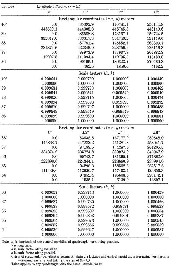
19. BONNE PROJECTION #
SUMMARY #
- Pseudoconical.
- Central meridian is a straight line. Other meridians are complex curves.
- Parallels are concentric circular arcs, but the poles are points.
- Scale is true along the central meridian and along all parallels.
- No distortion along the central meridian and along the standard parallel.
- Used for atlas maps of continents and for topographic mapping of some countries.
- Sinusoidal projection is equatorial limiting form of Bonne projection.
- Used considerably by Bonne in mid-18th century, but developed by others during the early 16th century.
HISTORY #
The name of Rigobert Bonne (1727-1795), a French geographer, is almost universally applied to an equal-area projection which has been used for both large- and small-scale mapping during the past 450 years. During the late 19th and early 20th centuries, the most conspicuous use of the Bonne projection was for maps of continents in atlases.
The Italian Bernardus Sylvanus’ world map of 1511 closely approaches the Bonne projection, since its meridians are almost equally spaced along the equidistant and concentric circular parallels. De l’Isle and Coronelli used the Bonne principle for maps of about 1700. Bonne used the projection most notably for a 1752 maritime atlas of the coast of France (Reignier, 1957, p. 164). Continental maps of Europe and Asia appeared on this projection by 1763, and the ellipsoidal version replaced the Cassini projection for French topographic mapping beginning in 1803.
For maps of continents, the Bonne was preceded by its polar limiting form, a cordiform (heart-shaped) world map devised by Johannes Stabius and given wider notice by Johannes Werner about 1514. The Werner projection, as it is usually called, was used in the late 16th century for maps of Asia and Africa by Mercator and Abraham Ortelius, but the “Bonne” projection has less distortion because its projection center is at the center of the region being mapped instead of at the pole. Eventually the Werner projection was made obsolete by the Bonne.
FEATURES AND USAGE #
Like the Equidistant Conic with one standard parallel, the Bonne projection (fig. 27) has concentric circular arcs for parallels of latitude. They are equally spaced on the spherical form and spaced in proportion to the true distance along a meridian on the ellipsoidal form. The chosen standard parallel is given its true curvature on the map by making the radius of its circular arc equal to the distance between the parallel and the apex of a cone tangent at the parallel. FIGURE 27.— Bonne projection with central parallel at lat. 40° N. Called a pseudoconic projection, this is equal-area and has no distortion along central meridian or central parallel. Popular in atlases for maps of continents until mid-20th century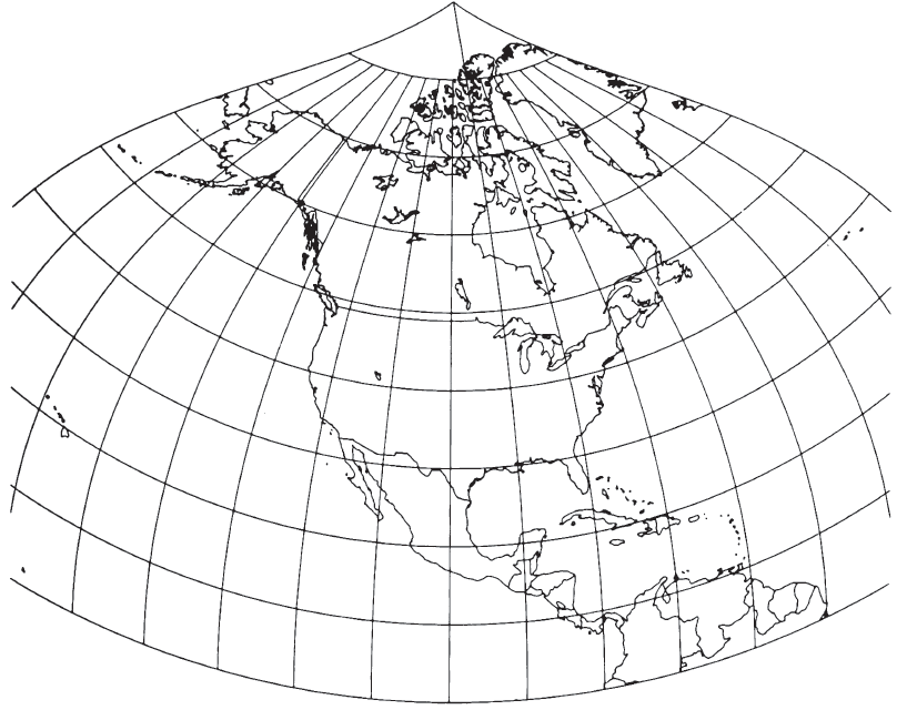
The combination of curved meridians and concentric circular arcs for parallels has led to the classification of “pseudoconic” for the Bonne projection and for the polar limiting case, the Werner projection, on which the North Pole is the equivalent of the standard parallel. The limiting case with the Equator as the standard parallel is the Sinusoidal, a “pseudocylindrical” projection to be discussed later; the formulas must be changed in this case since the parallels of latitude are straight. Modifications to the Bonne projection, in some cases resulting in nonequal-area projections, were presented by Nell of Germany in 1890 and by Solov’ev of the Soviet Union in the 1940’s (Maling, 1960, p. 295-296).
Many atlases of the 19th and early 20th centuries utilized the Bonne projection to show North America, Europe, Asia, and Australia, while the Sinusoidal (as the equatorial Bonne) was used for South America and Africa. The Lambert Azimuthal Equal-Area projection is now generally used by Rand McNally & Co. and Hammond Inc. for maps of continents, while the National Geographic Society prefers its own Chamberlin Trimetric projection for this purpose.
Large-scale use of the Bonne projection for topographic mapping, originally introduced by France, is current chiefly in portions of France, Ireland, Morocco, and some countries in the eastern Mediterranean area (Clifford J. Mugnier, written commun., 1985).
FORMULAS FOR THE SPHERE #
The principles stated above lead to the following forward formulas for rectangular coordinates of the spherical form of the Bonne projection, given $R, \phi_1, \lambda_0, \phi$ and $\lambda$, and using radians in equation (19-1),
The inverse formulas for the sphere, given $R, \phi_1, \lambda_0, x$, and $y$, to find $(\phi, \lambda)$:
FORMULAS FOR THE ELLIPSOID #
For the forward formulas, given $a, e, \phi_1, \lambda_0, \phi$, and $\lambda$, to find $x$ and $y$, the following are calculated in order:
For the inverse formulas for the ellipsoid, given $a, e, \phi_1, \lambda_0, x$ and $y$, to find $\phi$ and $\lambda$, first $m_1$, and $M_1$ are calculated as in the forward case from equations (14-15) and (3-21) above. The following are then calculated in order:
For Hawaii, the standard parallels are lats. 20° 40’ and 23° 20’ N.; the corresponding base map was not prepared for Alaska. ↩︎