20. ORTHOGRAPHIC PROJECTION #

SUMMARY #

Azimuthal.

All meridians and parallels are ellipses, circles, or straight lines.
Neither conformal nor equal-area.
Closely resembles a globe in appearance, since it is a perspective projection from infinite distance.
Only one hemisphere can be shown at a time.
Much distortion near the edge of the hemisphere shown.
No distortion at the center only.
Directions from the center are true.
Radial scale factor decreases as distance increases from the center.
Scale in the direction of the lines of latitude is true in the polar aspect.
Used chiefly for pictorial views.
Used only in the spherical form.
Known by Egyptians and Greeks 2,000 years ago.

HISTORY #

To the layman, the best known perspective azimuthal projection is the Orthographic, although it is the least useful for measurements. While its distortion in shape and area is quite severe near the edges, and only one hemisphere may be shown on a single map, the eye is much more willing to forgive this distortion than to forgive that of the Mercator projection because the Orthographic projection makes the map look very much like a globe appears, especially in the oblique aspect.

The Egyptians were probably aware of the Orthographic projection, and Hipparchus of Greece (2nd century B.C.) used the equatorial aspect for astronomical calculations. Its early name was “analemma,” a name also used by Ptolemy, but it was replaced by “orthographic” in 1613 by François d’Aiguillon of Antwerp. While it was also used by Indians and Arabs for astronomical purposes, it is not known to have been used for world maps older than 16th-century works by Albrecht Dürer (1471 - 1528), the German artist and cartographer, who prepared polar and equatorial versions (Keuning, 1955, p. 6).

FEATURES #

The point of perspective for the Orthographic projection is at an infinite distance, so that the meridians and parallels are projected onto the tangent plane with projection lines. All meridians and parallels are shown as ellipses, circles, or straight lines.

As on all polar azimuthal projections, the meridians of the polar Orthographic projection appear as straight lines radiating from the pole at their true angles, while the parallels of latitude are complete circles centered about the pole. On the Orthographic, the parallels are spaced most widely near the pole, and the spacing decreases to zero at the Equator, which is the circle marking the edge of the map (figs. 28, 29A). As a result, the land shapes near the pole are prominent, while lands near the Equator are compressed so that they can hardly be recognized. In spite of the fact that the scale along the meridians varies from the correct value at the pole to zero at the Equator, the scale along every parallel is true.

FIGURE 28.— Geometric projection of the parallels of the polar Orthographic projection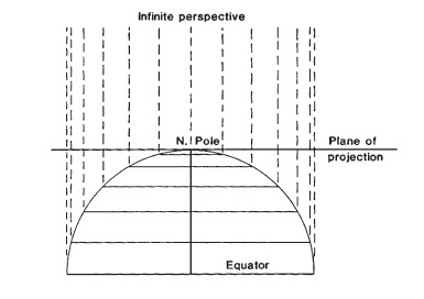 — **FIGURE 28**.— Geometric projection of the parallels of the polar Orthographic projection

The equatorial aspect of the Orthographic projection has as its center some point on the Earth’s Equator. Here, all the parallels of latitude including the Equator are seen edge-on; thus, they appear as straight parallel lines (fig. 29B). The meridians, which are shaped like circles on the sphere, are projected onto the map at various inclinations to the lines of perspective. The central meridian, seen edge-on, is a straight line. The meridian 90° from the central meridian is shown as a circle marking the limit of the equatorial aspect. This circle is equidistantly marked with parallels of latitude. Other meridians are ellipses of eccentricities ranging from zero (the bounding circle) to 1.0 (the central meridian).

The oblique Orthographic projection, with its center somewhere between the Equator and a pole, gives the classic globelike appearance; and in fact an oblique view, with its center near but not on the Equator or pole, is often preferred to the equatorial or polar aspect for pictorial purposes. On the oblique Orthographic, the only straight line is the central meridian, if it is actually portrayed. All parallels of latitude are ellipses with the same eccentricity (fig. 29C). Some of these ellipses are shown completely and some only partially, while some cannot be shown at all. All other meridians are also ellipses of varying eccentricities. No meridian appears as a circle on the oblique aspect.

The intersection of any given meridian and parallel is shown on an Orthographic projection at the same distance from the central meridian, regardless of whether the aspect is oblique, polar, or equatorial, provided the same central meridian and the same scale are maintained. Scale and distortion, as on all azimuthal projections, change only with the distance from the center. The center of projection has no distortion, but the outer regions are compressed, even though the scale is true along all circles drawn about the center. (These circles are not “standard” lines because the scale is true only in the direction followed by the line.)

FIGURE 29.— Orthographic projection. (A) Polar aspect. (B) Equatorial aspect, approximately the view of the Moon, Mars, and outer planets as seen from the Earth. (C) Oblique aspect, centered at 40° N., giving the classic globelike view. — **FIGURE 29**.— Orthographic projection. (A) Polar aspect. (B) Equatorial aspect, approximately the view of the Moon, Mars, and outer planets as seen from the Earth. (C) Oblique aspect, centered at 40° N., giving the classic globelike view.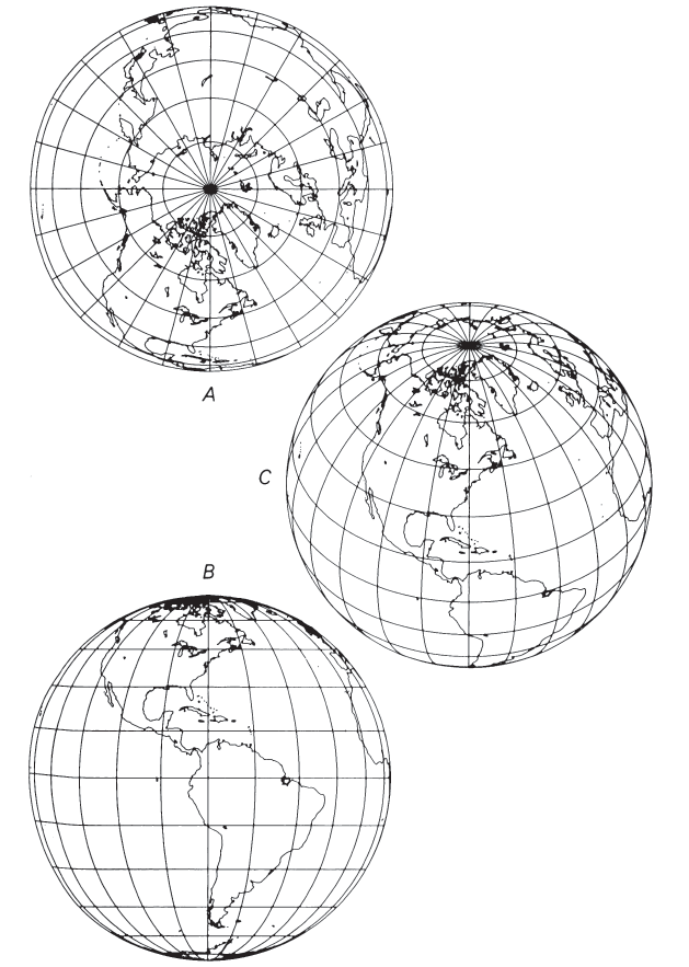

USAGE #

The Orthographic projection seldom appears in atlases, except as a globe in relief without meridians and parallels. When it does appear, it provides a striking view. Richard Edes Harrison has used the Orthographic for several maps in an atlas of the 1940’s partially based on this projection. Frank Debenham (1968) used photographed relief globes extensively in The Global Atlas, and Rand McNally has done likewise in their world atlases since 1960. The USGS has used it occasionally as a frontispiece or end map (USGS, 1970; Thompson, 1979), but it also provided a base for definitive maps of voyages of discovery across the North Atlantic (USGS, 1970, p. 133).

It became especially popular during the Second World War when there was stress on the global nature of the conflict. With some space fights of the 1960’s, the first photographs of the Earth from space renewed consciousness of the Orthographic concept.

GEOMETRIC CONSTRUCTION #

The three aspects of the Orthographic projection may be graphically constructed with an adaptation of the draftsman’s technique shown by Raisz (1962, p. 180). Referring to figure 30, circle A is drawn for the polar aspect, with meridians marked at true-angles. Perpendiculars are dropped from the intersections of the outer circle with the meridians onto the horizontal meridian EE. This determines the radii of the parallels of latitude, which may then be drawn about the center.

F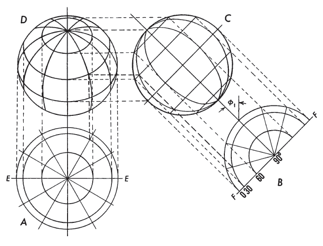or the equatorial aspect, circle C is drawn with the same radius as A, circle B is drawn like half of circle A, and the outer circle of C is equidistantly marked to locate intersections of parallels with that circle. Parallels of latitude are drawn as straight lines, with the Equator midway. Parallels are shown tilted merely for use with oblique projection circle D. Points at intersections of parallels with other meridians of B are then projected onto the corresponding parallels of latitude on C, and the new points connected for the meridians of C. By tilting graticule C at an angle $\phi_1$ equal to the central latitude of the desired oblique aspect, the corresponding points of circles A and C may be projected vertically and horizontally, respectively, onto circle D to provide intersections for meridians and parallels.

FORMULAS FOR THE SPHERE #

To understand the mathematical concept of the Orthographic projection, it is helpful to think in terms of polar coordinates $\rho$ and $\theta$:

$$ \rho = R\sin{c} \tag{ 20-1 } $$

$$ \theta = \pi-Az = 180^\circ-Az \tag{ 20-2 } $$

where $c$ is the angular distance of the given point from the center of projection. $Az$ is the azimuth east of north, and $\theta$ is the polar coordinate east of south. The distance from the center of a point on an Orthographic map projection is thus proportional to the sine of the angular distance from the center on the sphere. Applying equations (5-3), (5-4), and (5-4a) for great circle distance $c$ and azimuth $Az$ in terms of latitude and longitude, and equations for rectangular coordinates in terms of polar coordinates, the equations for rectangular coordinates for the oblique Orthographic projection reduce to the following, given $R, \phi_1, \lambda_0, \phi,$ and $\lambda$ (see numerical examples):

$$ x = R\cos\phi\sin{(\lambda - \lambda_0)} \tag{ 20-3 } $$

$$ y = R[\cos\phi_1\sin\phi - \sin\phi_1\cos\phi\cos{(\lambda - \lambda_0)}] \tag{ 20-4 } $$

$$ \begin {align} h' &= \cos{c} \\ &= \sin\phi_1\sin\phi+\cos\phi_1\cos\phi\cos{(\lambda-\lambda_0)} \\ k' &= 1.0 \end{align} \tag{ 20-5 } $$

where $\phi_1$, and $\lambda_0$ are the latitude and longitude, respectively, of the center point and origin of the projection, $h’$ is the scale factor along a line radiating from the center, and $k’$ is the scale factor in a direction perpendicular to a line radiating from the center. The Y axis coincides with the central meridian $\lambda_0$, y increasing northerly. All the parallels are ellipses of eccentricity $\cos\phi_1$. The limit of the map is a circle of radius $R$.

For the north polar Orthographic, letting $\phi_1=90°$, x is still found from (20-3), but

$$ y = -R\cos\phi\cos{(\lambda-\lambda_0)} \tag{ 20-6 } $$

$$ h = \sin\phi \tag{ 20-7 } $$

In polar coordinates,

$$ \rho = R\cos\phi \tag{ 20-8 } $$

$$ \theta = (\lambda-\lambda_0) \tag{ 20-9 } $$

For the south polar Orthographic, with $\phi = -90°$, x does not change, but

$$ y = R\cos\phi\cos{(\lambda-\lambda_0)} \tag{ 20-10 } $$

$$ h = -\sin\phi \tag{ 20-11 } $$

{For polar coordinates, $\rho$ is found from (20-8), but

$$ \theta = \pi - \lambda + \lambda_0 \tag{ 20-12 } $$

For the equatorial Orthographic, letting $\phi_1 = 0$, x still does not change from (20-3), but

$$ y = R\sin\phi \tag{ 20-13 } $$

In automatically computing a general set of coordinates for a complete Orthographic map, the distance $c$ from the center should be calculated for each intersection of latitude and longitude to determine whether it exceeds 90° and therefore whether the point is beyond the range of the map. More directly, using equation (5-3),

$$ \cos c = \sin\phi_1\sin\phi + \cos\phi_1\cos\phi\cos{(\lambda-\lambda_0)} \tag{ 5-3 } $$

if $\cos{c}$ is zero or positive, the point is to be plotted. If $\cos{c}$ is negative, the point is not to be plotted. For the inverse formulas for the sphere, to find $\phi$ and $\lambda$, given $R, \phi_1, \lambda_0, x,$ and $y$:

$$ \phi = \arcsin{[\cos{c}\sin\phi_1+(y\sin{c}\cos\phi_1/\rho)]} \tag{ 20-14 } $$

If $\rho = 0$, equations (20-14) through (20-17) are indeterminate, but $\phi = \phi_1$, and $\lambda = \lambda_0$. If $\phi_1$ is not $\pm90°$,

$$ \lambda = \lambda_0 + \arctan{[x\sin{c}/(\rho\cos\phi_1\cos{c}-y\sin\phi_1\sin{c})]} \tag{ 20-15 } $$

If $\phi_1$ is 90°,

$$ \lambda = \lambda_0+\arctan{[x/(-y)]} \tag{ 20-16 } $$

If $\phi_1$ is -90°,

$$ \lambda = \lambda_0 + \arctan{(x/y)} \tag{ 20-17 } $$

Note that, while the ratio $[x(-y)]$ in (20-16) is numerically the same as $(-x/y)$, the necessary quadrant adjustment is different when using the Fortran ATAN2 function or its equivalent.

In equations (20-14) and (20-15),

$$ \rho = (x^2+y^2)^{1/2} \tag{ 20-18 } $$

$$ c = \arcsin{(\rho/R)} \tag{ 20-19 } $$

Simplification for inverse equations for the polar and equatorial aspects is obtained by giving $\phi_1$, values of $\pm90°$ and $0°$, respectively. They are not given in detail here.

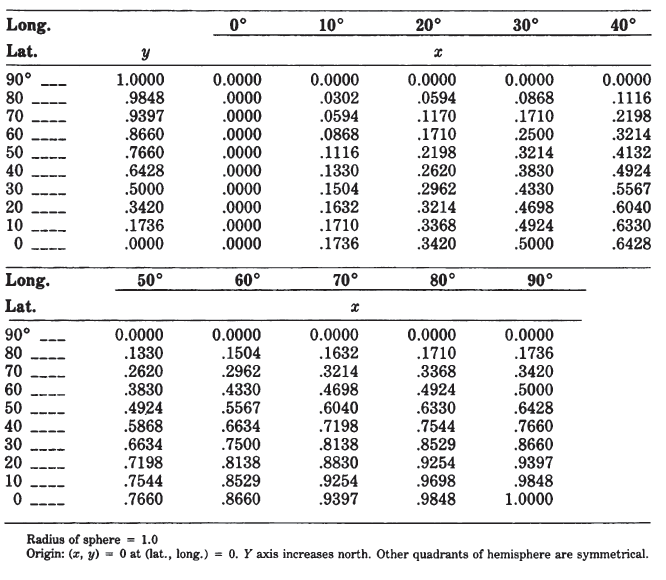
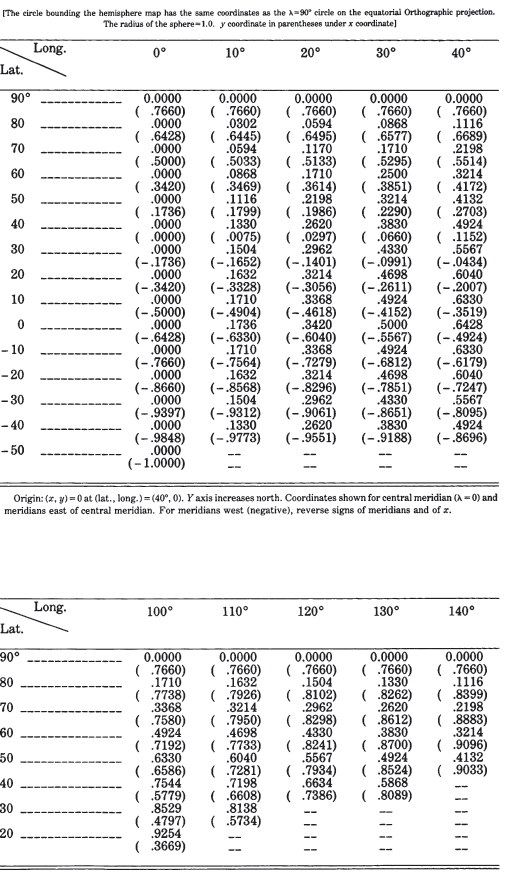
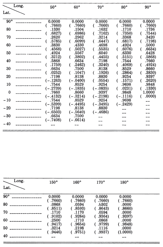
Tables 22 and 23 list rectangular coordinates for the equatorial and oblique aspects, respectively, for a 10° graticule with a sphere of radius $R = 1.0$. For the oblique example $\phi_1 = 40°$.

TABLE 22.— Orthographic projection: Rectangular coordinates for equatorial aspect — **TABLE 22**.— Orthographic projection: Rectangular coordinates for equatorial aspect

TABLE 23.— Orthographic projection: Rectangular coordinates for oblique aspect centered at lat. 40° N. — **TABLE 23**.— Orthographic projection: Rectangular coordinates for oblique aspect centered at lat. 40° N.