24. LAMBERT AZIMUTHAL EQUAL-AREA PROJECTION #
SUMMARY #
- Azimuthal.
- Equal-Area.
- All meridians in the polar aspect, the central meridian in other aspects, and the Equator in the equatorial aspect are straight lines.
- The outer meridian of a hemisphere in the equatorial aspect (for the sphere) and the parallels in the polar aspect (sphere or ellipsoid) are circles.
- All other meridians and parallels are complex curves.
- Not a perspective projection.
- Scale decreases radially as the distance increases from the center, the only point without distortion.
- Scale increases in the direction perpendicular to radii as the distance increases from the center.
- Directions from the center are true for the sphere and the polar ellipsoidal forms.
- Point opposite the center is shown as a circle surrounding the map (for the sphere).
- Used for maps of continents and hemispheres.
- Presented by Lambert in 1772.
HISTORY #
The last major projection presented by Johann Heinrich Lambert in his 1772 Beiträge was his azimuthal equal-area projection (Lambert, 1772, p. 75-78). His name is usually applied to the projection in modem references, but it is occasionally called merely the Azimuthal (or Zenithal) Equal-Area projection. Not only is it equal-area, with, of course, the azimuthal property showing true directions from the center of the projection, but its scale at a given distance from the center varies less from the scale at the center than the scale of any of the other major azimuthals (see table 21).
Lambert discussed the polar and equatorial aspects of the Azimuthal Equal-Area projection, but the oblique aspect is just as popular now. The polar aspect was apparently independently derived by Lorgna in Italy in 1789, and the latter was called the originator in a publication a century later (USC&GS, 1882, p. 290). G. A. Ginzburg proposed two modifications of the general Lambert Azimuthal projection in 1949 to reduce the angular distortion at the expense of creating a slight distortion in area (Maling, 1960, p. 206). A common modification was devised by Ernst Hammer in 1892 and is called the Hammer or Hammer-Aitoff projection. It consists of halving the vertical coordinates of the equatorial aspect of one hemisphere and doubling the values of the meridians from center. It retains equality of area, but it is no longer azimuthal.
FEATURES #
The Lambert Azimuthal Equal-Area projection is not a perspective projection. It may be called a “synthetic” azimuthal in that it was derived for the specific purpose of maintaining equal area. The ellipsoidal form maintains equal area, but it is not quite azimuthal except in the polar aspect, so the name for the general ellipsoidal form is a slight misnomer, although it looks like the spherical azimuthal form and has most of its other characteristics.
The polar aspect (fig. 39A), like that of the Orthographic and Stereographic, has circles for parallels of latitude, all centered about the North or South Pole, and straight equally spaced radii of these circles for meridians. The difference is, once again, in the spacing of the parallels. For the Lambert, the spacing between the parallels gradually decreases with increasing distance from the pole. The opposite pole, not visible on either the Orthographic or Stereographic, may be shown on the Lambert as a large circle surrounding the map, almost half again as far as the Equator from the center. Normally, the projection is not shown beyond one hemisphere (or beyond the Equator in the polar aspect).
The equatorial aspect (fig. 39B) has, like the other azimuthals, a straight Equator and straight central meridian, with a circle representing the 90th meridian east and west of the central meridian. Unlike those for the Orthographic and Stereographic, the remaining meridians and parallels are uncommon complex curves. The chief visual distinguishing characteristic is that the spacing of the meridians near the 90th meridian and sf the parallels near the poles is about 0.7 of the spacing at the center of the projection, or moderately less to the eye. The parallels of latitude look considerably like circular arcs, except near the 90th meridians, where they exhibit a noticeable turn toward the nearest pole.
The oblique aspect (fig. 39C) of the Lambert Azimuthal Equal-Area resembles the Orthographic to some extent, until it is seen that crowding is far less pronounced as the distance from the center increases. Aside from the straight central meridian, all meridians and parallels are complex curves, not ellipses.
In both the equatorial and oblique aspects, the point opposite the center may be shown as a circle surrounding the map, corresponding to the opposite pole in the polar aspect. Except for the advantage of showing the entire Earth in an equal-area projection from one point, the distortion is so great beyond the inner hemisphere that for world maps the Earth should be shown as two separate hemispherical maps, the second map centered on the point opposite the center of the first map. FIGURE 39.— Lambert Azimuthal Equal-Area projection. (A) Polar aspect showing one hemisphere; the entire globe may be included in a circle of 1.41 times the diameter of the Equator. (B) Equatorial aspect; frequently used in atlases for maps of the Eastern and Western hemispheres. (C) Oblique aspect; centered on lat. 40° N.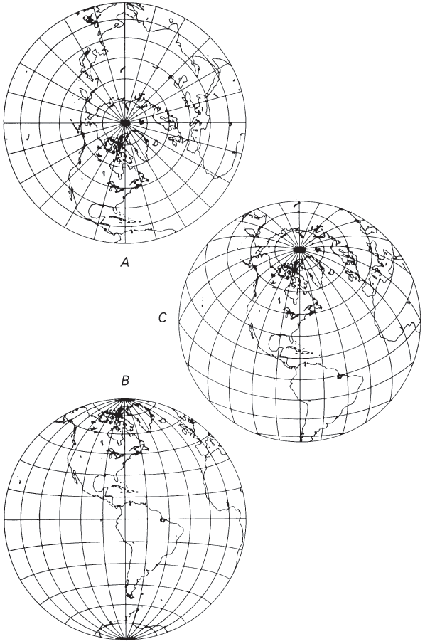
USAGE #
The spherical form in all three aspects of the Lambert Azimuthal Equal-Area projection has appeared in recent commercial atlases for Eastern and Western Hemispheres (replacing the long-used Globular projection) and for maps of oceans and most of the continents and polar regions.
The polar aspect appears in the National Atlas (USGS, 1970, p. 148-149) for maps delineating north and south polar expeditions, at a scale of 1:39,000,000. It is used at a scale of 1:20,000,000 for the Arctic Region as an inset on the 1978 USGS Map of Prospective Hydrocarbon Provinces of the World.
The USGS has prepared six base maps of the Pacific Ocean on the spherical form of the Lambert Azimuthal Equal-Area. Four sections, at 1:10,000,000, have centers at 35° N., 150° E. ; 35° N., 135° W.; 35° S., 135° E.; and 40° S., 100° W. The Pacific-Antarctic region, at a scale of 1:8,300,000, is centered at 20° S. and 165° W., while a Pacific Basin map at 1:17,100,000 is centered at the Equator and 160° W. (The last two maps were originally erroneously labeled with scales that are too small.) The base maps have been used for individual geographic, geologic, tectonic, minerals, and energy maps. The USGS has also cooperated with the National Geographic Society in revising maps of the entire Moon drawn to the spherical form of the equatorial Lambert Azimuthal Equal-Area.
GEOMETRIC CONSTRUCTION #
The polar aspect (for the sphere) may be drawn with a simple geometric construction: In figure 40, if angle AOR is the latitude $\phi$ and P is the pole at the center, PA is the radius of that latitude on the polar map. The oblique and equatorial aspects have no direct geometric construction. They may be prepared indirectly by using other azimuthal projections (Harrison, 1943), but it is now simpler to plot automatically or manually from rectangular coordinates which are generated by a relatively simple computer program. The formulas are given below. FIGURE 40.— Geometric construction of polar Lambert Azimuthal Equal-Area projection.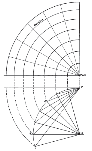
FORMULAS FOR THE SPHERE #
On the Lambert Azimuthal Equal-Area projection for the sphere, a point at a given angular distance from the center of projection is plotted at a distance from the center proportional to the sine of half that angular distance, and at its true azimuth, or
For the north polar Lambert Azimuthal Equal-Area, with $\phi_1=90^\circ$, since $k’$ is $k$ for the polar aspect, these formulas simplify to the following (see numerical examples):
If $\rho = 0$, equations (20-14) through (20-17) are indeterminate, but $\phi = \phi_1$, and $\lambda = \lambda_0$. If $\phi_1$ is not $\pm90°$,
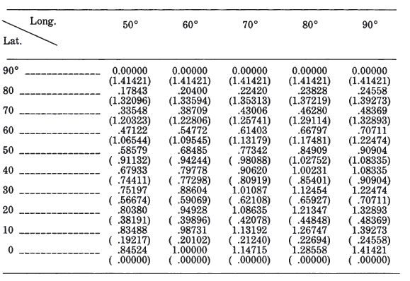
Table 28 lists rectangular coordinates for the equatorial aspect for a 10° graticule with a sphere of radius $R = 1.0$. TABLE 28.— Lambert Azimuthal Equal-Area projection: Rectangular coordinates for equatorial aspect (sphere)
FORMULAS FOR THE ELLIPSOID #
As noted above, the ellipsoidal oblique aspect of the Lambert Azimuthal Equal-Area projection is slightly nonazimuthal in order to preserve equality of area. To date, the USGS has not used the ellipsoidal form in any aspect. The formulas are analogous to the spherical equations, but involve replacing the geodetic latitude $\phi$ with authalic latitude $\beta$ (see equation (3-11)). In order to achieve correct scale in all directions at the center of projection, that is, to make the center a “standard point,” a slight adjustment using $D$ is also necessary. The general forward formulas for the oblique aspect are as follows, given $a, e, \phi_1, \lambda_0, \phi,$ and $\lambda$ (see numerical examples):
For the south polar aspect, $(\phi_1 = -90^\circ)$, equations (21-30) and (21-32) remain the same, but
The inverse formulas for the polar aspects involve relatively simple transformations of above equations (21-30), (21-31), and (24-23), except that $\phi$ is found from the iterative equation (3-16), listed just above, in which $q$ is calculated as follows:
TABLE 29.— Ellipsoidal polar Lambert Azimuthal Equal-Area projection (International ellipsoid)