25. AZIMUTHAL EQUIDISTANT PROJECTION #

SUMMARY #

Azimuthal.
Distances measured from the center are true.
Distances not measured along radii from the center are not correct.
The center of projection is the only point without distortion.
Directions from the center are true (except on some oblique and equatorial ellipsoidal forms).
Neither equal-area nor conformal.
All meridians on the polar aspect, the central meridian on other aspects, and the Equator on the equatorial aspect are straight lines.
Parallels on the polar projection are circles spaced at true intervals (equidistant for the sphere).
The outer meridian of a hemisphere on the equatorial aspect (for the sphere) is a circle.
All other meridians and parallels are complex curves.
Not a perspective projection.
Point opposite the center is shown as a circle (for the sphere) surrounding the map.
Used in the polar aspect for world maps and maps of polar hemispheres.
Used in the oblique aspect for atlas maps of continents and world maps for aviation and radio use.
Known for many centuries in the polar aspect.

HISTORY #

While the Orthographic is probably the most familiar azimuthal projection, the Azimuthal Equidistant, especially in its polar form, has found its way into many atlases with the coming of the air age for maps of the Northern and Southern Hemispheres or for world maps. The simplicity of the polar aspect for the sphere, with equally spaced meridians and equidistant concentric circles for parallels of latitude, has made it easier to understand than most other projections. The primary feature, showing distances and directions correctly from one point on the Earth’s surface, is also easily accepted. In addition, its linear scale distortion is moderate and falls between that of equal-area and conformal projections.

Like the Orthographic, Stereographic, and Gnomonic projections, the Azimuthal Equidistant was apparently used centuries before the 15th-century surge in scientific mapmaking. It is believed that Egyptians used the polar aspect for star charts, but the oldest existing celestial map on the projection was prepared in 1426 by Conrad of Dyffenbach. It was also used in principle for small areas by mariners from earliest times in order to chart coasts, using distances and directions obtained at sea.

The first clear examples of the use of the Azimuthal Equidistant for polar maps of the Earth are those included by Gerardus Mercator as insets on his 1569 world map, which introduced his famous cylindrical projection. As Northern and Southern Hemispheres, the projection appeared in a manuscript of about 1510 by the Swiss Henricus Loritus, usually called Glareanus (1488-1563), and by several others in the next few decades (Keuning, 1955, p. 4-5). Guillaume Postel is given credit in France for its origin, although he did not use it until 1581. Antonio Cagnoli even gave the projection his name as originator in 1799 (Deetz and Adams, 1934, p. 163; Steers, 1970, p. 234). Philippe Hatt developed ellipsoidal versions of the oblique aspect which are used by the French and the Greeks for coastal or topographic mapping.

Two projections with similar names are called the Two-Point Azimuthal and the Two-Point Equidistant projections. Both were developed about 1920 independently by Maurer (1919) of Germany and Close (1921) of England. The first projection (rarely used) is geometrically a tilting of the Gnomonic projection to provide true azimuths from either of two chosen points instead of from just one. Like the Gnomonic; it shows all great circle arcs as straight lines and is limited to one hemisphere. The Two-Point Equidistant has received moderate use and interest, and shows true distances, but not true azimuths, from either of two chosen points to any other point on the map, which may be extended to show the entire world (Close, 1934).

The Chamberlin Trimetric projection is an approximate “three-point equidistant” projection, constructed so that distances from three chosen points to any other point on the map are approximately correct. The latter distances cannot be exactly true, but the projection is a compromise which the National Geographic Society uses as a standard projection for maps of most continents. This projection was geometrically constructed by the Society, of which Wellman Chamberlin (1908-76) was chief cartographer for many years.

An ellipsoidal adaptation of the Two-Point Equidistant was made by Jay K. Donald of American Telephone and Telegraph Company in 1956 to develop a grid still used by the Bell Telephone system for establishing the distance component of long distance rates. Still another approach is Bomford’s modification of the Azimuthal Equidistant, in which the usual circles of constant scale factor perpendicular to the radius from the center are made ovals to give a better average scale factor on a map with a rectangular border (Lewis and Campbell, 1951, p. 7, 12-15).

FEATURES #

The Azimuthal Equidistant projection, like the Lambert Azimuthal Equal-Area, is not a perspective projection, but in the spherical form, and in some of the ellipsoidal forms, it has the azimuthal characteristic that all directions or azimuths are correct when measured from the center of the projection. As its special feature, all distances are at true scale when measured between this center and any other point on the map.

The polar aspect (fig. 41A), like other polar azimuthals, has circles for parallels of latitude, all centered about the North or South Pole, and equally spaced radii of these circles for meridians. The parallels are, however, spaced equidistantly on the spherical form (or according to actual parallel spacings on the ellipsoid). A world map can extend to the opposite pole, but distortion becomes infinite. Even though the map is finite, the point for the opposite pole is shown as a circle twice the radius of the mapped Equator, thus giving an infinite scale factor along that circle. Likewise, the countries of the outer hemisphere are visibly increasingly distorted as the distance from the center increases, while the inner hemisphere has little enough distortion to appear rather satisfactory to the eye, although the east-west scale along the Equator is almost 60 percent greater than the scale at the center.

As on other azimuthals, there is no distortion at the center of the projection and, as on azimuthals other than the Stereographic, the scale cannot be reduced at the center to provide a standard circle of no distortion elsewhere. It is possible to use an average scale over the map involved to minimize variations in scale error in any direction, but this defeats the main purpose of the projection, that of providing true distance from the center. Therefore, the scale at the projection center should be used for any Azimuthal Equidistant map.

The equatorial aspect (fig. 41B) is least used of the three Azimuthal Equidistant aspects, primarily because there are no cities along the Equator from which distances in all directions have been of much interest to map users. Its potential use as a map of the Eastern or Western Hemisphere was usually supplanted first by the equatorial Stereographic projection, later by the Globular projection (both graticules drawn entirely with arcs of circles and straight lines), and now by the equatorial Lambert Azimuthal Equal-Area.

For the equatorial Azimuthal Equidistant projection of the sphere, the only straight lines are the central meridian and the Equator. The outer circle for one hemisphere (the meridian 90" east and west of the central meridian) is equidistantly marked off for the parallels, as it is on other azimuthals. The other meridians and parallels are complex curves constructed to maintain the correct distances and azimuths from the center. The parallels cross the central meridian at their true equidistant spacings, and the meridians cross the Equator equidistantly. The map can be extended, like the polar aspect, to include a much-distorted second hemisphere on the same center.

The oblique Azimuthal Equidistant projection (fig. 41C) rather resembles the oblique Lambert Azimuthal Equal-Area when confined to the inner hemisphere centered on any chosen point between Equator and pole. Except for the straight central meridian, the graticule consists of complex curves, positioned to maintain true distance and azimuth from the center. When the outer hemisphere is included, the difference between the Equidistant and the Lambert becomes more pronounced, and while distortion is as extreme as in other aspects, the distances and directions of the features from the center now outweigh the distortion for many applications.

FIGURE 41.— Azimuthal Equidistant projection. (A) Polar aspect extending to the South Pole; commonly used in atlases for polar maps. (B) Equatorial aspect. (C) Oblique aspect centered on lat. 40° N. Distance from the center is true to scale.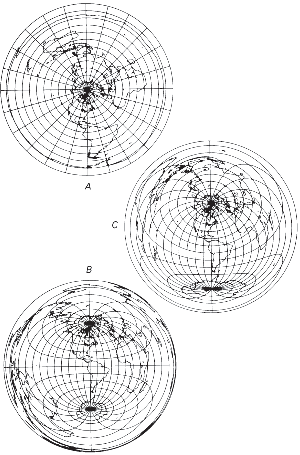 — **FIGURE 41**.— Azimuthal Equidistant projection. (A) Polar aspect extending to the South Pole; commonly used in atlases for polar maps. (B) Equatorial aspect. (C) Oblique aspect centered on lat. 40° N. Distance from the center is true to scale.

USAGE #

The polar aspect of the Azimuthal Equidistant has regularly appeared in commercial atlases issued during the past century as the most common projection for maps of the north and south polar areas. It is used for polar insets on Van der Grinten-projection world maps published by the National Geographic Society and used as base maps (including the insets) by USGS. The polar Azimuthal Equidistant projection is also normally used when a hemisphere or complete sphere centered on the North or South Pole is to be shown. The oblique aspect has been used for maps of the world centered on important cities or sites and occasionally for maps of continents. Nearly all these maps use the spherical form of the projection.

The USGS has used the Azimuthal Equidistant projection in both spherical and ellipsoidal form. An oblique spherical version of the Earth centered at lat. 40° N., long. 100° W., appears in the National Atlas (USGS, 1970, p. 329). At a scale of 1:175,000,000, it does not show meridians and parallels, but shows circles at 1,000-mile intervals from the center. The ellipsoidal oblique aspect is used for the plane coordinate projection system in approximate form for Guam and in nearly rigorous form for islands in Micronesia.

GEOMETRIC CONSTRUCTION #

The polar Azimuthal Equidistant is among the easiest projections to construct geometrically, since the parallels of latitude are equally spaced in the spherical case and the meridians are drawn at their true angles. There are no direct geometric constructions for the oblique and equatorial aspects. Like the Lambert Azimuthal Equal-Area, they may be prepared indirectly by using other azimuthal projections (Harrison, 1943), but automatic computer plotting or manual plotting of calculated rectangular coordinates is the most suitable means now available.

FORMULAS FOR THE SPHERE #

On the Azimuthal Equidistant projection for the sphere, a given point is plotted at a distance from the center of the map proportional to the distance on the sphere and at its true azimuth, or

$$ \rho = R\,c \tag{ 25-1 } $$

$$ \theta = \pi-Az = 180^\circ-Az \tag{ 20-2 } $$

where $c$ is the angular distance from the center, $Az$ is the azimuth east of north (see equations (5-3) through (5-4b)), and $\theta$ is the polar coordinate east of south. For k’ and h’, see equation (25-2) and the statement below. Combining various equations, the rectangular coordinates for the oblique Azimuthal Equidistant projection are found as follows, given $R, \phi_1, \lambda_0, \phi,$ and $\lambda$ (see numerical examples):

$$ x = R\,k'\,\cos\phi\sin(\lambda-\lambda_0) \tag{ 22-4 } $$

$$ y = R\,k'\,[\cos\phi_1\sin\phi-\sin\phi_1\cos\phi\cos(\lambda-\lambda_0)] \tag{ 22-5 } $$

where

$$ k' = c/\sin{c} \tag{ 25-2 } $$

$$ \cos c = \sin\phi_1\sin\phi + \cos\phi_1\cos\phi\cos{(\lambda-\lambda_0)} \tag{ 5-3 } $$

and $(\phi_1,\lambda_0)$ are latitude and longitude of the center of projection and origin. The Y axis coincides with the central meridian $\lambda_0$ and y increases northerly. If $\cos{c}= 1$, equation (25-2) is indeterminate, but $k’ = 1$, and $x = y = 0$. If $\cos{c} = -1$, the point opposite the center $(-\phi_1, \lambda_0\pm180^\circ)$ is indicated; it is plotted as a circle of radius $\pi R$. The term $k’$ is the scale factor in a direction perpendicular to the radius from the center of the map, not along the parallel, except in the polar aspect. The scale factor $h’$ in the direction of the radius is 1.0.

For the north polar aspect, with $\phi_1 = 90^\circ$,

$$ x = R(\pi/2-\phi)\sin(\lambda-\lambda_0) \tag{ 25-3 } $$

$$ y = -R(\pi/2-\phi)\cos(\lambda-\lambda_0) \tag{ 25-4 } $$

$$ k = (\pi/2-\phi)/\cos\phi \tag{ 25-5 } $$

$$ h = 1.0 $$

$$ \rho = R(\pi/2-\phi) \tag{ 25-6 } $$

$$ \theta = (\lambda-\lambda_0) \tag{ 20-9 } $$

For the south polar aspect, with $\phi_1 = -90^\circ$

$$ x = R(\pi/2+\phi)\sin(\lambda-\lambda_0) \tag{ 25-7 } $$

$$ y = -R(\pi/2+\phi)\cos(\lambda-\lambda_0) \tag{ 25-8 } $$

$$ k = (\pi/2+\phi)/\cos\phi \tag{ 25-9 } $$

$$ h = 1.0 $$

$$ \rho = R(\pi/2+\phi) \tag{ 25-10 } $$

$$ \theta = \pi - \lambda + \lambda_0 \tag{ 20-12 } $$

For the equatorial aspect, with $\phi_1 = 0$, $x$ is found from (22-4) and $k$’ from (25-2), but

$$ y = R\,k'\sin\phi \tag{ 25-11 } $$

and

$$ \cos{c} = \cos\phi\cos(\lambda-\lambda_0) \tag{ 25-12 } $$

The maximum angular deformation $\omega$ for any of these aspects, using equations (4-7) through (4-9), since $h’ = 1.0$:

$$ \begin{align} \sin{\omega/2} &= (k'-1)(k'+1)\tag{25-13} \cr &= (c-\sin{c})/(c+\sin{c}) \tag{25-14} \end{align} $$

For the inverse formulas for the sphere, given $R, \phi_1, \lambda_0, x,$ and $y$:

$$ \phi = \arcsin{[\cos{c}\sin\phi_1+(y\sin{c}\cos\phi_1/\rho)]} \tag{ 20-14 } $$

If $\rho = 0$, equations (20-14) through (20-17) are indeterminate, but $\phi = \phi_1$, and $\lambda = \lambda_0$.

If $\phi_1$ is not $\pm90°$:

$$ \lambda = \lambda_0 + \arctan{[x\sin{c}/(\rho\cos\phi_1\cos{c}-y\sin\phi_1\sin{c})]} \tag{ 20-15 } $$

If $\phi_1$ is 90°,

$$ \lambda = \lambda_0+\arctan{[x/(-y)]} \tag{ 20-16 } $$

If $\phi_1$ is -90°,

$$ \lambda = \lambda_0 + \arctan{(x/y)} \tag{ 20-17 } $$

In equations (20-14) and (20-15),

$$ \rho = (x^2+y^2)^{1/2} \tag{ 20-18 } $$

$$ c = \rho/R \tag{ 25-15 } $$

Except for (25-15), the above inverse formulas are the same as those for the other azimuthals, and (25-2) is the only change from previous azimuthals among the general (oblique) formulas (22-4) through (5-3) for the forward calculations as listed above.

Table 30 shows rectangular coordinates for the equatorial aspect for a 10° graticule with a sphere of radius $R = 1.0$.

TABLE 30.— Azimuthal Equidistant projection: Rectangular coordinates for equatorial aspect (sphere) — **TABLE 30**.— Azimuthal Equidistant projection: Rectangular coordinates for equatorial aspect (sphere)

FORMULAS FOR THE ELLIPSOID #

The formulas for the polar aspect of the ellipsoidal Azimuthal Equidistant projection are relatively simple and are theoretically accurate for a map of the entire world. However, such a use is unnecessary because the errors of the sphere versus the ellipsoid become insignificant when compared to the basic errors of projection. The polar form is truly azimuthal as well as equidistant. Given $a, e, \lambda_0, \phi_1, \phi,$ and $\lambda$, for the north polar aspect, $\phi_1 = 90^\circ$ (numerical examples):

$$ x = \rho\sin(\lambda-\lambda_0) \tag{ 21-30 } $$

$$ y = -\rho\cos(\lambda-\lambda_0) \tag{ 21-31 } $$

$$ k = \rho/(a m) \tag{ 21-32 } $$

where

$$ \rho = M_p-M \tag{ 25-16 } $$

$$ \eqalign { M = a[ &(1-e^2/4-3e^4/64-5e^6/256-\dots)\phi \cr - &(3e^2/8+3e^4/32+45e^6/1024+\dots)\sin{2\phi} \cr + &(15e^4/256+45e^6/1024+\dots)\sin{4\phi} - (35e^6/3072+\dots)\sin{6\phi}+\dots] } \tag{ 3-21 } $$

with $M_p$ the value of $M$ for $\phi$ of 90°, and

$$ m = \cos\phi/(1-e^2\sin^2\phi)^{1/2} \tag{ 14-15 } $$

For improved computational efficiency using this series, see p. 19. For the south polar aspect, the equations for the north polar aspect apply, except that equations (21-31) and (25-16) become

$$ y = \rho \cos(\lambda-\lambda_0) \tag{ 24-24 } $$

$$ \rho = M_p+M \tag{ 25-17 } $$

The origin falls at the pole in either case, and the Y axis follows the central meridian $\lambda_0$. For the north polar aspect, $\lambda_0$ is shown below the pole, and y increases along ho toward the pole. For the south polar aspect, $\lambda$, is shown above the pole, and y increases along ho away from the pole.

Table 31 lists polar coordinates for the ellipsoidal aspect of the Azimuthal Equidistant, using the International ellipsoid.

TABLE 31.— Ellipsoidal Azimuthal Equidistant projection (International ellipsoid)—Polar Aspect — **TABLE 31**.— Ellipsoidal Azimuthal Equidistant projection (International ellipsoid)—Polar Aspect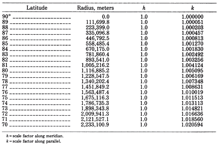

For the oblique and equatorial aspects of the ellipsoidal Azimuthal Equidistant, both nearly rigorous and approximate sets of formulas have been derived. For mapping of Guam, the National Geodetic Survey and the USGS use an approximation to the ellipsoidal oblique Azimuthal Equidistant called the “Guam projection.” It is described by Claire (1968, p. 52-53) as follows (changing his symbols to match those in this publication):

The plane coordinates of the geodetic stations on Guam were obtained by first computing the geodetic distances [$c$] and azimuths [$Az$] of all points from the origin by inverse computations. The coordinates were then computed by the equations: [$x = c \sin {Az}$ and $y = c \cos {Az}$]. This really gives a true azimuthal equidistant projection. The equations given here are simpler, however, than those for a geodetic inverse computation, and the resulting coordinates computed using them will not be significantly different from those computed rigidly by inverse computation. This is the reason it is called an approximate azimuthal equidistant projection.

The formulas for the Guam projection are equivalent to the following:

$$ x = a(\lambda-\lambda_0)\cos\phi/(1-e^2\sin^2\phi)^{1/2} \tag{ 25-18 } $$

$$ y = M - M_1 + x^2 \tan\phi(1-e^2\sin^2\phi)^{1/2}/(2a) \tag{ 25-19 } $$

where $M$ and $M_1$ are found from equation (3-21) for $\phi$ and $\phi_1$ Actually, the original formulas are given in terms of seconds of rectifying latitude and geodetic latitude and longitude, but they may be written as above. The $x$ coordinate is thus taken as the distance along the parallel, and $y$ is the distance along the central meridian $\lambda_0$ with adjustment for curvature of the parallel. The origin occurs at $(\phi_1, \lambda_0)$, the Y axis coincides with the central meridian, and y increases northerly.

For Guam, $\phi_1 = 13^\circ28'20.87887’’$ N. lat. and $\lambda_0 = 144^\circ44'55.50254’’$ E. long., with 50,000 m added to both $x$ and $y$ to eliminate negative numbers. The Clarke 1866 ellipsoid is used. The above formulas provide coordinates within 5 mm at full scale of those using ellipsoidal Polyconic formulas for the region of Guam.

A more complicated and more accurate approach to the oblique ellipsoidal Azimuthal Equidistant projection is used for plane coordinates of various individual islands of Micronesia. In this form, the true distance and azimuth of any point on the island or in nearby waters are measured from the origin chosen for the island and along the normal section or plane containing the perpendicular to the surface of the ellipsoid at the origin. This is not exactly the same as the shortest or geodesic distance between the points, but the difference is negligible (Bomford, 1971, p. 125). This distance and azimuth are plotted on the map. The projection is, therefore, equidistant and azimuthal with respect to the center and appears to satisfy all the requirements for an ellipsoidal Azimuthal Equidistant projection, although it is described as a “modified” form. The origin is assigned large-enough values of x and y to prevent negative readings.

The formulas for calculation of this distance and azimuth have been published in various forms, depending on the maximum distance involved. The projection system for Micronesia makes use of “Clarke’s best formula” and Robbins’ inverse of this. These are considered suitable for lines up to 800 km in length. The formulas below, rearranged slightly from Robbins’ formulas as given in Bomford (1971, p. 136-137), are extended to produce rectangular coordinates. No iteration is required. They are listed in the order of use, given a central point at lat. $\phi_1$, long. $\lambda_0$, coordinates $x_0$ and $y_0$ of the central point, the Y axis along the central meridian $\lambda_0$, y increasing northerly, ellipsoidal parameters $a$ and $e$, and $\phi$ and $\lambda$.

To find $x$ and $y$:

$$ N_1 = a/(1-e^2\sin^2{\phi_1})^{1/2} \tag{ 4-20a } $$

$$ N = a/(1-e^2\sin^2{\phi})^{1/2} \tag{ 4-20 } $$

$$ \psi = \arctan[(1-e^2)\tan\phi+e^2N_1\sin\phi_1/(N\cos\phi)] \tag{ 25-20 } $$

$$ Az = \arctan\{\sin(\lambda-\lambda_0)/[\cos\phi_1\tan\psi - \sin\phi_1\cos(\lambda-\lambda_0)]\} \tag{ 25-21 } $$

The ATAN2 Fortran function should be used with equation (25-21), but it is not applicable to (25-20). If $\sin{Az} = 0$,

$$ s = \pm\arcsin(\cos\phi_1\sin\psi - \sin\phi_1\cos\psi) \tag{ 25-22 } $$

taking the sign of $\cos{Az}$.

If $\sin{Az} \ne 0$,

$$ s = \arcsin[\sin(\lambda-\lambda_0)\cos\psi/\sin{Az}] \tag{ 25-22a } $$

In either case,

$$ G = e\sin\phi_1/(1-e^2)^{1/2} \tag{ 25-23 } $$

$$ H = e\cos\phi_1\cos{Az}/(1-e^2)^{1/2} \tag{ 25-24 } $$

$$ \begin{align} c = &N_1s\{1-s^2H^2(1-H^2)/6 + (s^3/8)GH(1-2H^2) \cr &+(s^4/120)[H^2(4-7H^2)-3G^2(1-7H^2)]-(s^5/48)GH\} \end{align} \tag{ 25-25 } $$

$$ x = c\sin{Az} + x_0 \tag{ 25-26 } $$

$$ y = c\cos{Az} + y_0 \tag{ 25-27 } $$

where $c$ is the geodesic distance, and $Az$ is azimuth east of north.

Table 32 shows the parameters for the various islands mapped with this projection.

TABLE 32.— Plane coordinate systems for Micronesia: Clarke 1866 ellipsoid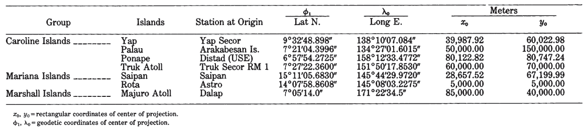 — **TABLE 32**.— Plane coordinate systems for Micronesia: Clarke 1866 ellipsoid

Inverse formulas for the polar ellipsoidal aspect, given $a, e, \phi_1, \lambda_0, x,$ and $y$:

$$ \begin{align} \phi = \mu &+ (3e_1/2-27e_1^3/32+\dots)\sin{2\mu}+(21e_1^2/16-55e_1^4/32+\dots)\sin{4\mu} \\ &+ (151e_1^3/96-\dots)\sin{6\mu}+(1097e_1^4/512-\dots)\sin{8\mu}+\dots \end{align} \tag{ 3-26 } $$

where

$$ e_1 = [1-(1-e^2)^{1/2}]/[1+(1-e^2)^{1/2}] \tag{ 3-24 } $$

$$ \mu=M/[a(1-e^2/4-3e^4/64-5e^6/256-\dots)] \tag{ 7-19 } $$

$$ M = M_p - \rho \text{ for the north polar case} \tag{ 25-28 } $$

and

$$ M=\rho - M_p \text{ for the south polar case} \tag{ 25-29 } $$

For improved computational efficiency using series (3-26) see p. 19. Equation (3-21), listed with the forward equations, is used to find $M_p$ for $\phi = 90^\circ$. For either case,

$$ \rho = (x^2+y^2)^{1/2} \tag{ 20-18 } $$

For longitude, for the north polar case,

$$ \lambda = \lambda_0+\arctan[x/(-y)] \tag{ 20-16 } $$

For the south polar case,

$$ \lambda = \lambda_0+\arctan[x/y] \tag{ 20-17 } $$

Inverse formulas for the Guam projection (Claire, 1968, p. 53) involve an iteration of two equations, which may be rearranged and rewritten in the following form consistent with the above formulas. Given $a, e, \phi_1, \lambda_0, x,$ and $y$, $M_1$ is calculated for $\phi_1$, from (3-21), given with forward equations. (If false northings and eastings are included in $x$ and $y$, they must be subtracted first.) Then, first assuming $\phi = \phi_1$,

$$ M = M_1 + y - x^2\tan\phi(1-e^2\sin^2\phi)^{1/2}/(2a) \tag{ 25-30 } $$

Using this $M$, $\mu$ is calculated from (7-19) and inserted into the right side of (3-26) to solve for a new $\phi$ on the left side. This is inserted into (25-30), a new $M$ is found, and it is resubstituted into (7-19), $\mu$ into (3-26), etc., until $\phi$ on the left side of (3-26) changes by less than a chosen convergence figure, for a final $\phi$. Then

$$ \lambda = \lambda_0 + x(1-e^2\sin^2\phi)^{1/2}/(a\cos\phi) \tag{ 25-31 } $$

The inverse Guam formulas arbitrarily stop at three iterations, which are sufficient for the small area.

For the Micronesia version of the ellipsoidal Azimuthal Equidistant projection, the inverse formulas given below are “Clarke’s best formula,” as given in Bomford (1971, p. 133) and do not involve iteration. They have also been rearranged to begin with rectangular coordinates, but they are also suitable for finding latitude and longitude accurately for a point at any given distance $c$ (up to about 800 km) and azimuth $Az$ (east of north) from the center, if equations (25-32) and (25-33) are deleted. In order of use, given $a, e$, central point at lat. $\phi_1$, long. $\lambda_0$, rectangular coordinates of center $x_0, y_0$, and $x$ and $y$ for another point, to find $\phi$ and $\lambda$:

$$ c = [(x-x_0)^2+(y-y_0)^2]^{1/2} \tag{ 25-32 } $$

$$ Az = \arctan[(x-x_0)/(y-y_0)] \tag{ 25-33 } $$

$$ N_1 = a/(1-e^2\sin^2{\phi_1})^{1/2} \tag{4-20a} $$

$$ A = -e^2\cos^2\phi_1\cos^2{Az}/(1-e^2) \tag{ 25-34 } $$

$$ B = 3e^2 (1-A)\sin\phi_1\cos\phi_1cos{Az}/(1-e^2) \tag{ 25-35 } $$

$$ D = c/N_1 \tag{ 25-36 } $$

$$ E = D - A(1+A)D^3/6-B(1+3A)D^4/24 \tag{ 25-37 } $$

$$ F = 1-AE^2/2 - BE^3/6 \tag{ 25-38 } $$

$$ \psi = \arcsin(\sin\phi_1\cos{E}+\cos\phi_1\sin{E}\cos{Az}) \tag{ 25-39 } $$

$$ \lambda = \lambda_0+\arcsin(\sin{Az}\sin{E}/\cos\psi) \tag{ 25-40 } $$

$$ \phi = \arctan[(1-e^2F\sin\phi_1/\sin\psi)\tan\psi/(1-e^2)] \tag{ 25-41 } $$

The ATAN2 function of Fortran, or equivalent, should be used in equation (25-33), but not (25-41).

To convert coordinates measured on an existing Azimuthal Equidistant map (or other azimuthal map projection), the user may choose any meridian for $\lambda_0$ on the polar aspect, but only the original meridian and parallel may be used for $\lambda_0$ and $\phi_1$ respectively, on other aspects.