26. MODIFIED-STEREOGRAPHIC CONFORMAL PROJECTIONS #
SUMMARY #
- Modified azimuthal.
- Conformal.
- All meridians and parallels are normally complex curves, although some may be straight under some conditions.
- Scale is true along irregular lines, but map is usually designed to minimize scale variation throughout a selected region.
- Map is normally not symmetrical about any axis or point.
- Used for maps of continents in the Eastern Hemisphere, for the Pacific Ocean, and for maps of Alaska and the 50 United States.
- Specific forms devised by Miller, Lee, and Snyder, 1950-84.
HISTORY AND USAGE #
Two short mathematical formulas, taken as a pair, absolutely define the conformal transformation of one surface onto another surface. These formulas are called the Cauchy-Riemann equations, after two 19th-century mathematicians who added rigorous analysis to principles developed in the middle of the 18th century by physicist D’Alembert. Much later, Driencourt and Laborde (1932, vol. 14, p. 242) presented a fairly simple series (equation (26-4) below without the R), involving complex algebra (with imaginary numbers), that fully satisfies the Cauchy-Riemann equations and permits the formation of an endless number of new conformal map projections when certain constants are changed.
The advantage of this series is that lines of constant scale may be made to follow one of a variety of patterns, instead of following the great or small circles of the common conformal projections. The disadvantage is that the length of the series and the computations become increasingly lengthy as the irregularity of the lines of constant scale increases, but this problem has decreased with the development of computers.
Laborde (1928; Reignier, 1957, p. 130) applied this transformation to the mapping of Madagascar, starting with the Oblique Mercator projection and applying the complex equation up to the third-order or cubic terms. Miller (1953) used the same order of complex equation, but began with an oblique Stereographic projection. His resulting map of Europe and Africa has oval lines of constant scale (fig. 42); this projection is called the Miller Oblated (or Prolated) Stereographic. He subsequently (Miller, 1955) prepared similar projections for Asia and Australia each precisely conformal, but he linked them with nonconformal “fill-in” projections to provide a continuous map (in several sheets) of the land masses of the Eastern Hemisphere.
FIGURE 42.— Miller Oblated Stereographic projection of Europe and Africa, showing oval lines of constant scale. Center of projection lat. 18° N., long. 20° E.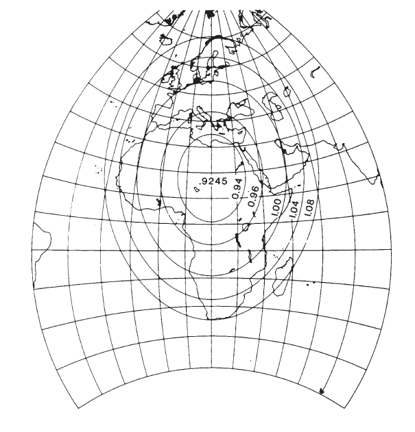
Lee (1974) designed a map of the Pacific Ocean, also using an oblique Stereographic with a third-order complex polynomial. The third-order polynomials used by Laborde, Miller, and Lee make relatively moderate computational demands, because several of the coefficients are zero, and the complex algebra can be readily simplified to equations without imaginary numbers. Recently Reilly (1973) and the writer (Snyder, 1984a, 1985a) have used much higher-order complex equations, but modern computers can readily handle them. Reilly used sixth-order coefficients with the regular Mercator for the new official New Zealand Map Grid, while the writer, beginning with oblique Stereographic projections, used sixth-order coefficients for a map of Alaska and tenth-order for a map of the 50 United States (figs. 43, 44). For these sixth- and tenth-order equations, only one coefficient is zero, but the other coefficients were computed using least squares. The projection for Alaska was used in 1985 by Alvaro F. Espinosa of the USGS to depict earthquake information for that State. The “Modified Transverse Mercator” projection is still being used by the USGS for most maps of Alaska.
FIGURE 43.— GS50 projection, with lines of constant scale factor superimposed. All 50 States, including islands and passages between Alaska, Hawaii, and the conterminous 48 States are shown with scale factors ranging only from 1.02 to 0.98.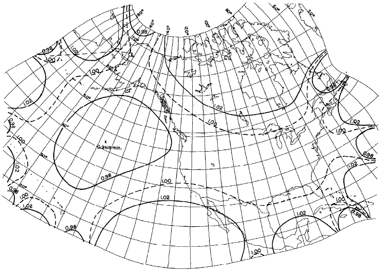
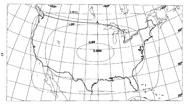
FIGURE 44.— Modified-Stereographic Conformal projection of Alaska, with lines of constant scale superimposed. Scale factors for Alaska range from 0.997 to 1.003, one-fourth the range for a corresponding conic projection. FIGURE 45.— Modified-Stereographic Conformal projection of 48 United States, bounded by a near-rectangle of constant scale. Three lines of constant scale are superimposed. Region bounded by near-rectangle has minimum error.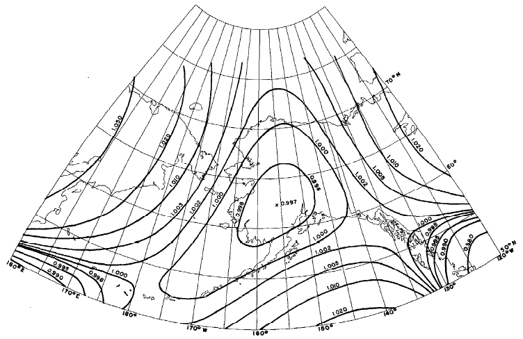
FEATURES #
The common feature linking the endless possibilities of map projections discussed in this chapter is the fact that they are perfectly conformal regardless of the order of the complex-algebra transformation, and regardless of the initial projection, provided it is also conformal.
Chebyshev (1856) stated that a region may be best shown conformally if the sum of the squares of the scale errors (scale factors minus 1) over the region is a minimum. He further declared that this results if the region is bounded by a line of constant scale. This was proven later. Thus the Stereographic is suitable for regions approximately circular in shape, but regions bounded by ovals, regular polygons, or rectangles may be mapped with nearly minimum error by suitably altering the Stereographic with the complex-algebra transformation.
If the region is irregular, such as Alaska, the region of interest may be divided into small elements, and the coefficients may be calculated using least squares to minimize the scale variation for the region shown. The resulting coefficients for the selected projections are given below, but the formulas for least-squares summation are not included here because they are lengthy and are only needed to devise new projections. For them the reader may refer to Snyder (1984a, 198413, 1985a).
The reduction of scale variation by using this complex-algebra transformation makes the ellipsoidal form even more important. This form is also simpler in these cases than for the Transverse Mercator and some other projections, because the lines of true scale normally do not follow a selected meridian, parallel, or other easily identifiable line in any case. Therefore, use of the conformal latitude in place of the geographic latitude is sufficient for the ellipsoidal form. This merely slightly shifts the lines of constant scale from one set of arbitrary locations to another. The coefficients have somewhat different values, however.
The meridians and parallels of the Modified-Stereographic projections are generally curved, and there is usually no symmetry about any point or line. There are limitations to these transformations. Most of them can only be used within a limited range, depending on the number and values of coefficients. As the distance from the projection center increases, the meridians, parallels, and shorelines begin to exhibit loops, overlapping, and other undesirable curves. A world map using the GS50 (50-State) projection is almost illegible, with meridians and parallels intertwined like wild vines.
Within the intended range of the map, the Modified-Stereographic projections can reduce the range of scale variation considerably when compared with standard conformal projections. The tenth-order complex-algebra modification used for the 50-State projection has a scale range of only ±2 percent (or 4 percent overall) for all 50 States placed in their relative geographical positions, including all islands, adjacent waters, water channels connecting Alaska, Hawaii, and the other 48 States, and nearby Canada and Mexico (fig. 43). A Lambert Conformal Conic projection previously used with standard parallels 37° and 65° N. to show the 50 States has a scale range of + 12 to -3 percent (or 15 percent overall). The sixth-order modification for the Alaska map, called the Modified-Stereographic Conformal projection, has a range of ±0.3 percent (or 0.6 percent overall) for Alaska itself, while a Lambert Conformal Conic with standard parallels 55° and 65° N. ranges from + 2.0 to -0.4 percent, or 2.4 percent overall.
The bounding of regions by ovals, near-regular polygons, or near-rectangles of constant scale results in improvement of scale variation by amounts depending on the size and shape of the boundary. The improvement in mean scale error is about 15 to 20 percent using a near-square instead of the circle of the base Stereographic projection. Using a Modified-Stereographic bounded by a near-rectangle instead of an oblique Mercator projection provides a mean improvement of up to 30 percent in some cases, but only 5 to 10 percent in cases involving a long narrow region. For fig. 45, the range of scale is ±1.1 percent (or 2.2 percent overall) within the 48 States, while the Lambert Conformal Conic normally used has a range of +2.4 to -0.6 percent (or 3.0 percent overall).
The improvement for the region in question is made at the expense of scale preservation outside the region. The regular conic projections maintain the same scale range around the entire world between the same latitude limits, even though most of that region is not shown on the regional maps described above.
FORMULAS FOR THE SPHERE #
The Modified-Stereographic conformal projections which have a scale range of more than 5 percent, such as regions bounded by rectangles 80° by 40° in spherical degrees, may satisfactorily be computed for the sphere instead of the ellipsoid. As stated above, development of coefficients is not shown here. For the calculation of final rectangular coordinates, given $R, \phi_1, \lambda_0, A_1$ through $A_m, B_1$ through $B_m$, $\phi,$ and $\lambda$, and to find $x$ and $y$ (see numerical examples):
For the practical computation of equations (26-4) and (26-5), Knuth’s (1969) algorithm is recommended instead of them. LetNote1
For inverse equations, given $R, \phi_1, \lambda_0, A_1$ through $A_m, B_1$ through $B_m$, $x$, and $y$, to find $\phi$ and $\lambda$, first a Newton-Raphson iteration may be used as follows to find $(x’ , y’)$:
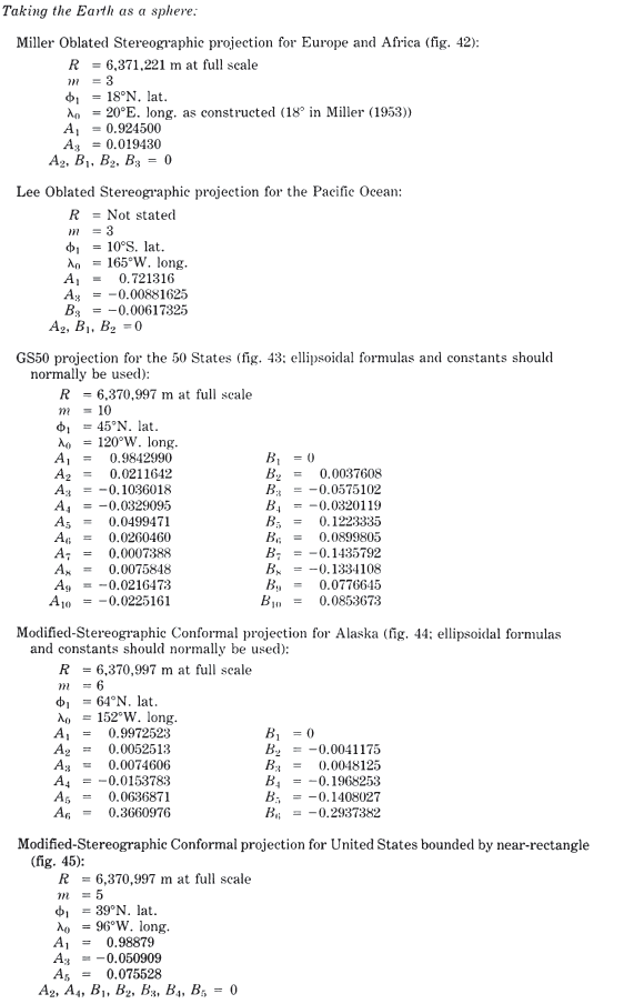
TABLE 33.— Modified-Stereographic Conformal projections: Coefficients for specific forms
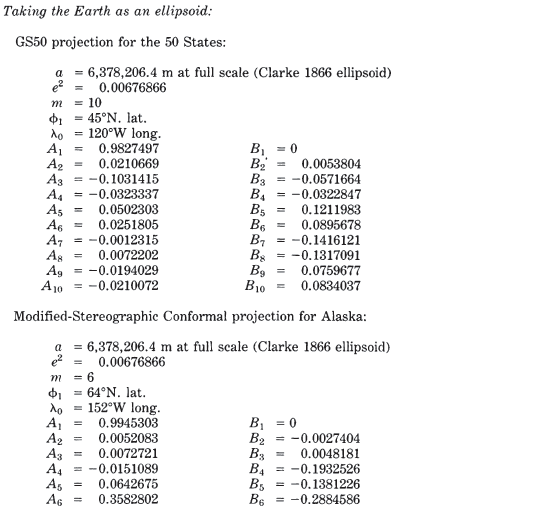
TABLE 33.— Modified-Stereographic Conformal projections: Coefficients for specific forms (Continued)
FORMULAS FOR THE ELLIPSOID #
For higher precision maps taking greater advantage of the reduced scale variation available with Modified-Stereographic Conformal projections, the ellipsoidal formulas should be used. Given $a, e, \phi_1, \lambda_0, A_1$ through $A_m, B_1$ through $B_m, \phi,$ and $\lambda$, to find $x$ and $y$ (special numerical examples are not given, but examples of the ellipsoidal Stereographic, and of the spherical Modified-Stereographic p. 344, are sufficiently similar):
For inverse equations, given $a, e, \phi_1,\lambda_0, A_1$ through $A_m, B_1$ through $B_m, x$, and $y$, to find $\phi$ and $\lambda$, the Newton-Raphson iteration of spherical equations (26-10) through (26-13) is used unchanged to find $(x’, y’)$ except that $R$ is replaced with $a$, and ellipsoidal constants must be used. After convergence, the final $(x’, y’)$ is converted to $(\phi$, \lambda)$ without iteration. Equations (26-14), (26-15), and (3-1) are used to calculate $\rho, c$, and $\chi_1$, as before. Then,
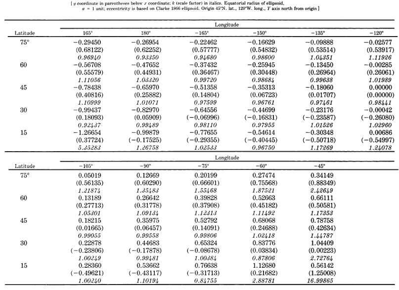
TABLE 34.— GS50 projection for 50 States: Rectangular coordinates for Clarke 1866 ellipsoid
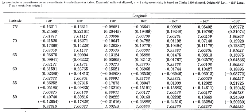
TABLE 35.— Modified-Stereographic Conformal projection for Alaska: Rectangular coordinates for Clarke 1866 ellipsoid