AZIMUTHAL AND RELATED MAP PROJECTIONS #
A third very important group of map projections, some of which have been known for 2,000 years, consists of five major azimuthal (or zenithal) projections and various less-common forms. While cylindrical and conic projections are related to cylinders and cones wrapped around the globe representing the Earth, the azimuthal projections are formed onto a plane which is usually tangent to the globe at either pole, the Equator, or any intermediate point. These variations are called the polar, equatorial (or meridian or meridional), and oblique (or horizon) aspects, respectively. Some azimuthals are true perspective projections; others are not. Although perspective cylindrical and conic projections are much less used than those which are not perspective, the perspective azimuthals are frequently used and have valuable properties. Complications arise when the ellipsoid is involved, but it is used only in special applications that are discussed below.
As stated earlier, azimuthal projections are characterized by the fact that the direction, or azimuth, from the center of the projection to every other point on the map is shown correctly. In addition, on the spherical forms, all great circles passing through the center of the projection are shown as straight lines. Therefore, the shortest route from this center to any other point is shown as a straight line. This fact made some of these projections especially popular for maps as flight and radio transmission became commonplace.
The five principal azimuthals are as follows:
- Orthographic. A true perspective, in which the Earth is projected from an infinite distance onto a plane. The map looks like a globe, thus stressing the roundness of the Earth.
- Stereographic. A true perspective in the spherical form, with the point of perspective on the surface of the sphere at a point exactly opposite the point of tangency for the plane, or opposite the center of the projection, even if the plane is secant. This projection is conformal for sphere or ellipsoid, but the ellipsoidal form is not truly perspective.
- Gnomonic. A true perspective, with the Earth projected from the center onto the tangent plane. All great circles, not merely those passing through the center, are shown as straight lines on the spherical form.
- Lambert Azimuthal Equal-Area. Not a true perspective. Areas are correct, and the overall scale variation is less than that found on the major perspective azimuthals.
- Azimuthal Equidistant. Not a true perspective. Distances from the center of the projection to any other point are shown correctly. Overall scale variation is moderate compared to the perspective azimuthals.
A sixth azimuthal projection of increasing interest in the space age is the general Vertical Perspective (resembling the Orthographic), projecting the Earth from any point in space, such as a satellite, onto a tangent or secant plant. It is used primarily in derivations and pictorial representations.
As a group, the azimuthals have unique esthetic qualities while remaining functional. There is a unity and roundness of the Earth on each (except perhaps the Gnomonic) which is not as apparent on cylindrical and conic projections.
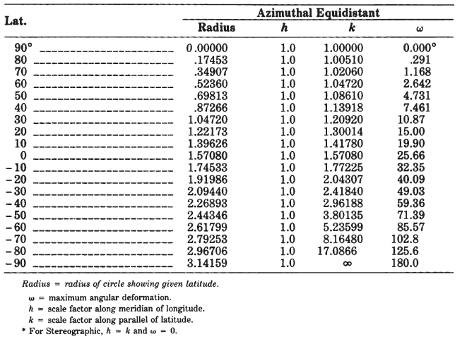
The simplest forms of the azimuthal projections are the polar aspects, in which all meridians are shown as straight lines radiating at their true angles from the center, while parallels of latitude are circles, concentric about the pole. The difference is in the spacing of the parallels. Table 21 lists for the five principal azimuthals the radius of every 10° of latitude on a sphere of radius 1.0 unit, centered on the North Pole. Scale factors and maximum angular deformation are also shown. The distortion is the same for the oblique and equatorial aspects at the same angular distance from the center of the projection, except that h and k are along and perpendicular to, respectively, radii from the center, not necessarily along meridians or parallels.
There are two principal drawbacks to the azimuthals. First, they are more difficult to construct than the cylindricals and the conics, except for the polar aspects. This drawback was more applicable, however, in the days before computers and plotters, but it is still more difficult to prepare a map having complex curves between plotted coordinates than it is to draw the entire graticule with circles and straight lines. Nevertheless, an increased use of azimuthal projections in atlases and for other published maps may be expected.
Secondly, most azimuthal maps do not have standard parallels or standard meridians. Each map has only one standard point: the center (except for the Stereographic, which may have a standard circle). Thus, the azimuthals are suitable for minimizing distortion in a somewhat circular region such as Antarctica, but not for an area with predominant length in one direction. TABLE 21.— Comparison of major azimuthal projections: Radius, scale factors, maximum angular distortion for projection of sphere with radius 1.0, North Polar aspect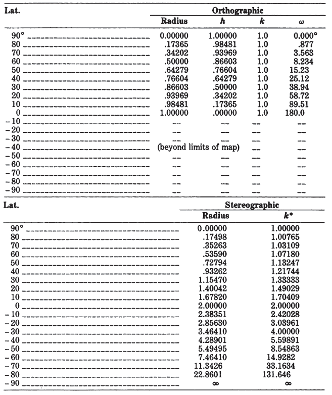

20. ORTHOGRAPHIC PROJECTION #
SUMMARY #
Azimuthal.
- All meridians and parallels are ellipses, circles, or straight lines.
- Neither conformal nor equal-area.
- Closely resembles a globe in appearance, since it is a perspective projection from infinite distance.
- Only one hemisphere can be shown at a time.
- Much distortion near the edge of the hemisphere shown.
- No distortion at the center only.
- Directions from the center are true.
- Radial scale factor decreases as distance increases from the center.
- Scale in the direction of the lines of latitude is true in the polar aspect.
- Used chiefly for pictorial views.
- Used only in the spherical form.
- Known by Egyptians and Greeks 2,000 years ago.
HISTORY #
To the layman, the best known perspective azimuthal projection is the Orthographic, although it is the least useful for measurements. While its distortion in shape and area is quite severe near the edges, and only one hemisphere may be shown on a single map, the eye is much more willing to forgive this distortion than to forgive that of the Mercator projection because the Orthographic projection makes the map look very much like a globe appears, especially in the oblique aspect.
The Egyptians were probably aware of the Orthographic projection, and Hipparchus of Greece (2nd century B.C.) used the equatorial aspect for astronomical calculations. Its early name was “analemma,” a name also used by Ptolemy, but it was replaced by “orthographic” in 1613 by François d’Aiguillon of Antwerp. While it was also used by Indians and Arabs for astronomical purposes, it is not known to have been used for world maps older than 16th-century works by Albrecht Dürer (1471 - 1528), the German artist and cartographer, who prepared polar and equatorial versions (Keuning, 1955, p. 6).
FEATURES #
The point of perspective for the Orthographic projection is at an infinite distance, so that the meridians and parallels are projected onto the tangent plane with projection lines. All meridians and parallels are shown as ellipses, circles, or straight lines.
As on all polar azimuthal projections, the meridians of the polar Orthographic projection appear as straight lines radiating from the pole at their true angles, while the parallels of latitude are complete circles centered about the pole. On the Orthographic, the parallels are spaced most widely near the pole, and the spacing decreases to zero at the Equator, which is the circle marking the edge of the map (figs. 28, 29A). As a result, the land shapes near the pole are prominent, while lands near the Equator are compressed so that they can hardly be recognized. In spite of the fact that the scale along the meridians varies from the correct value at the pole to zero at the Equator, the scale along every parallel is true. FIGURE 28.— Geometric projection of the parallels of the polar Orthographic projection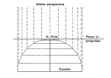
The equatorial aspect of the Orthographic projection has as its center some point on the Earth’s Equator. Here, all the parallels of latitude including the Equator are seen edge-on; thus, they appear as straight parallel lines (fig. 29B). The meridians, which are shaped like circles on the sphere, are projected onto the map at various inclinations to the lines of perspective. The central meridian, seen edge-on, is a straight line. The meridian 90° from the central meridian is shown as a circle marking the limit of the equatorial aspect. This circle is equidistantly marked with parallels of latitude. Other meridians are ellipses of eccentricities ranging from zero (the bounding circle) to 1.0 (the central meridian).
The oblique Orthographic projection, with its center somewhere between the Equator and a pole, gives the classic globelike appearance; and in fact an oblique view, with its center near but not on the Equator or pole, is often preferred to the equatorial or polar aspect for pictorial purposes. On the oblique Orthographic, the only straight line is the central meridian, if it is actually portrayed. All parallels of latitude are ellipses with the same eccentricity (fig. 29C). Some of these ellipses are shown completely and some only partially, while some cannot be shown at all. All other meridians are also ellipses of varying eccentricities. No meridian appears as a circle on the oblique aspect.
The intersection of any given meridian and parallel is shown on an Orthographic projection at the same distance from the central meridian, regardless of whether the aspect is oblique, polar, or equatorial, provided the same central meridian and the same scale are maintained. Scale and distortion, as on all azimuthal projections, change only with the distance from the center. The center of projection has no distortion, but the outer regions are compressed, even though the scale is true along all circles drawn about the center. (These circles are not “standard” lines because the scale is true only in the direction followed by the line.) FIGURE 29.— Orthographic projection. (A) Polar aspect. (B) Equatorial aspect, approximately the view of the Moon, Mars, and outer planets as seen from the Earth. (C) Oblique aspect, centered at 40° N., giving the classic globelike view.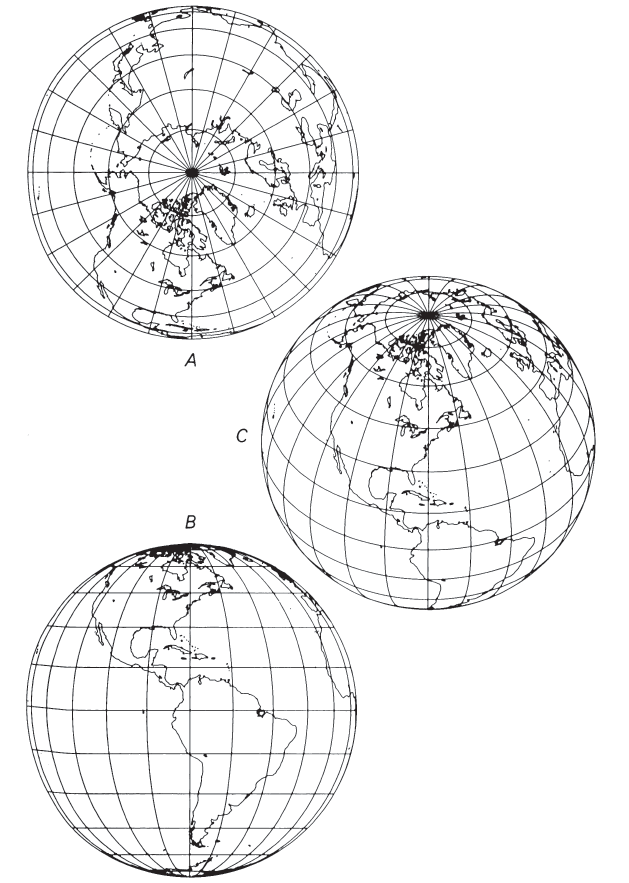
USAGE #
The Orthographic projection seldom appears in atlases, except as a globe in relief without meridians and parallels. When it does appear, it provides a striking view. Richard Edes Harrison has used the Orthographic for several maps in an atlas of the 1940’s partially based on this projection. Frank Debenham (1968) used photographed relief globes extensively in The Global Atlas, and Rand McNally has done likewise in their world atlases since 1960. The USGS has used it occasionally as a frontispiece or end map (USGS, 1970; Thompson, 1979), but it also provided a base for definitive maps of voyages of discovery across the North Atlantic (USGS, 1970, p. 133).
It became especially popular during the Second World War when there was stress on the global nature of the conflict. With some space fights of the 1960’s, the first photographs of the Earth from space renewed consciousness of the Orthographic concept.
GEOMETRIC CONSTRUCTION #
The three aspects of the Orthographic projection may be graphically constructed with an adaptation of the draftsman’s technique shown by Raisz (1962, p. 180). Referring to figure 30, circle A is drawn for the polar aspect, with meridians marked at true-angles. Perpendiculars are dropped from the intersections of the outer circle with the meridians onto the horizontal meridian EE. This determines the radii of the parallels of latitude, which may then be drawn about the center. FIGURE 30.— Geometric construction of polar, equatorial, and oblique Orthographic projections.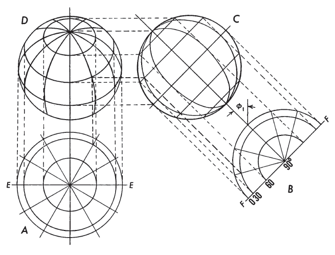
For the equatorial aspect, circle C is drawn with the same radius as A, circle B is drawn like half of circle A, and the outer circle of C is equidistantly marked to locate intersections of parallels with that circle. Parallels of latitude are drawn as straight lines, with the Equator midway. Parallels are shown tilted merely for use with oblique projection circle D. Points at intersections of parallels with other meridians of B are then projected onto the corresponding parallels of latitude on C, and the new points connected for the meridians of C. By tilting graticule C at an angle $\phi_1$ equal to the central latitude of the desired oblique aspect, the corresponding points of circles A and C may be projected vertically and horizontally, respectively, onto circle D to provide intersections for meridians and parallels.
FORMULAS FOR THE SPHERE #
To understand the mathematical concept of the Orthographic projection, it is helpful to think in terms of polar coordinates $\rho$ and $\theta$:
For the north polar Orthographic, letting $\phi_1=90°$, x is still found from (20-3), but
In equations (20-14) and (20-15),
Simplification for inverse equations for the polar and equatorial aspects is obtained by giving $\phi_1$, values of $\pm90°$ and $0°$, respectively. They are not given in detail here.
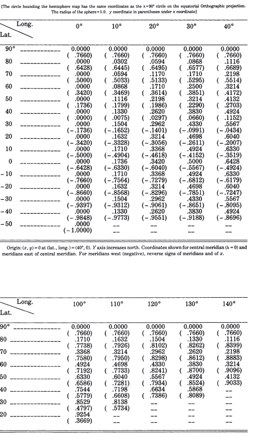
Tables 22 and 23 list rectangular coordinates for the equatorial and oblique aspects, respectively, for a 10° graticule with a sphere of radius $R = 1.0$. For the
oblique example $\phi_1 = 40°$. TABLE 22.— Orthographic projection: Rectangular coordinates for equatorial aspect TABLE 23.— Orthographic projection: Rectangular coordinates for oblique aspect centered at lat. 40° N.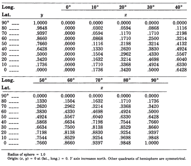
21. STEREOGRAPHIC PROJECTION #
SUMMARY #
- Azimuthal.
- Conformal.
- The central meridian and a particular parallel (if shown) are straight lines.
- All meridians on the polar aspect and the Equator on the equatorial aspect are straight lines.
- All other meridians and parallels are shown as arcs of circles.
- A perspective projection for the sphere.
- Directions from the center of the projection are true (except on ellipsoidal oblique and equatorial aspects).
- Scale increases away from the center of the projection.
- Point opposite the center of the projection cannot be plotted.
- Used for polar maps and miscellaneous special maps.
- Apparently invented by Hipparchus (2nd century B.C.).
HISTORY #
The Stereographic projection was probably known in its polar form to the Egyptians, while Hipparchus was apparently the first Greek to use it. He is generally considered its inventor. Ptolemy referred to it as “Planisphaerum,” a name used into the 16th century. The name “Stereographic” was assigned to it by François d’Aiguillon in 1613. The polar Stereographic was exclusively used for star maps until perhaps 1507, when the earliest-known use for a map of the world was made by Walther Ludd (Gaultier Lud) of St. Dié, Lorraine.
The oblique aspect was used by Theon of Alexandria in the fourth century for maps of the sky, but it was not proposed for geographical maps until Stabius and Werner discussed it together with their cordiform (heart-shaped) projections in the early 16th century. The earliest-known world maps were included in a 1583 atlas by Jacques de Vaulx (c. 1555-97). The two hemispheres were centered on Paris and its opposite point, respectively.
The equatorial Stereographic originated with the Arabs, and was used by the Arab astronomer Ibn-el-Zarkali (1029-87) of Toledo for an astrolabe. It became a basis for world maps in the early 16th century, with the earliest-known examples by Jean Roze (or Rotz), a Norman, in 1542. After Rumold (the son of Gerardus) Mercator’s use of the equatorial Stereographic for the world maps of the atlas of 1595, it became very popular among cartographers (Keuning, 1955, p. 7-9; Nordenskiold, 1889, p. 90, 92-93).
FEATURES #
Like the Orthographic, the Stereographic projection is a true perspective in its spherical form. It is the only known true perspective projection of any kind that is also conformal. Its point of projection is on the surface of the sphere at a point just opposite the point of tangency of the plane or the center point of the projection (fig. 31). Thus, if the North Pole is the center of the map, the projection is from the South Pole. All of one hemisphere can be comfortably shown, but it is impossible to show both hemispheres in their entirety from one center. The point on the sphere opposite the center of the map projects at an infinite distance in the plane of the map. FIGURE 31.— Geometric projection of the polar Stereographic projection.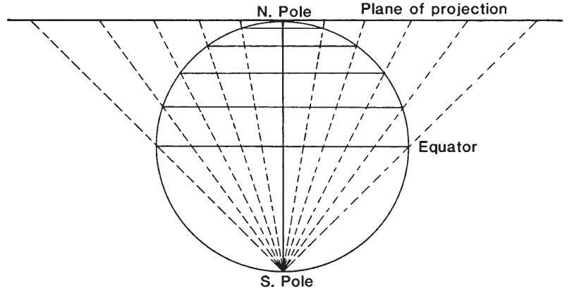
The polar aspect somewhat resembles other polar azimuthals, with straight radiating meridians and concentric circles for parallels (fig. 32A). The parallels are spaced at increasingly wide distances, the farther the latitude is from the pole (the Orthographic has the opposite feature).
In the equatorial and oblique aspects, the distinctive appearance of the Stereographic becomes more evident: All meridians and parallels, except for two, are shown as circles, and the meridians intersect the parallels at right angles (figs. 32B, C). The central meridian is shown straight, as is the parallel of the same numerical value, but opposite in sign to the central parallel. For example, if lat. 40° N. is the central parallel, then lat. 40° S. is shown as a straight line. For the equatorial aspect with lat. 0° as the central parallel, the Equator, which is of course also its own negative counterpart, is shown straight. (For the polar aspect, this has no meaning since the opposite pole cannot be shown.) Circles for parallels are centered along the central meridian; circles for meridians are centered along the straight parallel. The meridian 90° from the central meridian on the equatorial aspect is shown as a circle bounding the hemisphere. This circle is centered on the projection center and is equidistantly marked for parallels of latitude.
As an azimuthal projection, directions from the center are shown correctly in the spherical form. In the ellipsoidal form, only the polar aspect is truly azimuthal, but it is not perspective, in order to retain conformality. The oblique and equatorial aspects of the ellipsoidal Stereographic, in order to be conformal, are neither azimuthal nor perspective. As with other azimuthal projections, there is no distortion at the center, which may be made the “standard point” true to scale in all directions. Because of the conformality of the projection, a Stereographic map may be given, instead of a “standard point,” a “standard circle” (or “standard parallel” in the polar aspect) with an appropriate radius from the center, balancing the scale error throughout the map. (On the ellipsoidal oblique or equatorial aspects, the lines of constant scale are not perfect circles.) This cannot be done with non-conformal azimuthal projections. The Stereographic may also be modified to produce oval and irregular lines of true scale (see p. 203). FIGURE 32.— Stereographic projection. (A) Polar aspect; the most common scientific projection for polar areas of Earth, Moon, and the planets, since it is conformal. (B) Equatorial aspect; often used in the 16th and 17th centuries for maps of hemispheres. (C) Oblique aspect; centered on lat. 40° N. The Stereographic is the only geometric projection of the sphere which is conformal.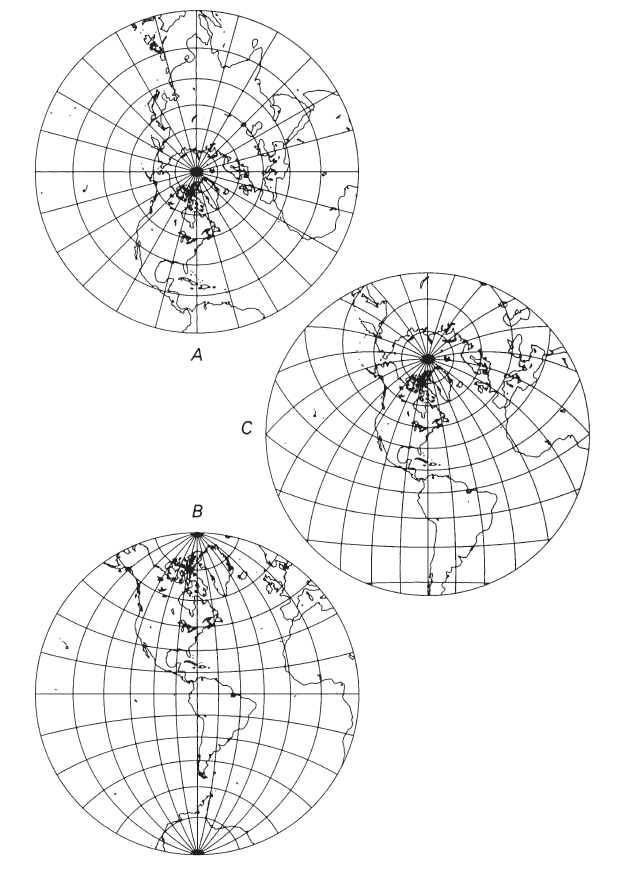
USAGE #
The oblique aspect of the Stereographic projection has been recently used in the spherical form by the USGS for circular maps of portions of the Moon, Mars, and Mercury, generally centered on a basin. The USGS is currently using the spherical oblique aspect to prepare 1:10,000,000-scale maps of Hydrocarbon Provinces for three continents after a least-squares analysis of over 100 points on each continent to determine optimum parameters for a common conformal projection. For Europe, the central scale factor is 0.976 at a central point of lat. 55°N. and long. 20°E. For Africa, these parameters are 0.941, 5° N., and 20° E. For Asia, they are 0.939, 45° N., and 105° E., respectively.
The USGS has most often wed the Stereographic in the polar aspect and ellipsoidal form for maps of Antarctica. For 1:500,000 sketch maps, the standard parallel is 71° S.; for its 1:250,000-scale series between 80° and the South Pole, the standard parallel is 80°14’ S. The Universal Transverse Mercator (UTM) grid employs the UPS (Universal Polar Stereographic) projection from the North Pole to lat. 84° N., and from the South Pole to lat. 80° S. For the UPS, the scale at each pole is reduced to 0.994, resulting in a standard parallel of 81°06'52.3" N. or S. The UPS central meridian (as defined for $\lambda_0$ on p. ix) is the Greenwich meridian, with false eastings and northings of 2,000,000 m at each pole.
In 1962, a United Nations conference changed the polar portion of the International Map of the World (at a scale of 1:1,000,000) from a modified Polyconic to the polar Stereographic. This has consequently affected IMW sheets drawn by the USGS. North of lat. 84° N. or south of lat. 80° S., it is used “with scale matching that of the Modified Polyconic Projection or the Lambert Conformal Conic Projection at Latitudes 84° N. and 80° S.” (United Nations, 1963, p. 10). The reference ellipsoid for all these polar Stereographic projections is the International of 1924.
The Astrogeology Center of the Geological Survey at Flagstaff, Ariz., has been using the polar Stereographic for the mapping of polar areas of every planet and satellite for which there is sufficient information in this region (see table 6).
The USGS is preparing a geologic map of the Arctic regions, using as a base an American Geographical Society map of the Arctic at a scale of 1:5,000,000. Drawn to the Stereographic projection, the map is based on a sphere having a radius which gives it the same volume as the International ellipsoid, and lat. 71° N. is made the standard parallel.
FORMULAS FOR THE SPHERE #
Mathematically, a point at a given angular distance from the chosen center point on the sphere is plotted on the Stereographic projection at a distance from the center proportional to the trigonometric tangent of half that angular distance, and at its true azimuth, or, if the central scale factor is 1,
If $\phi = -\phi_1$, and $\lambda=\lambda_0\pm180^\circ$, the point cannot be plotted. Geometrically, it is the point from which projection takes place. For the north polar Stereographic, with $\phi_1=90°$, these simplify to
TABLE 24.— Stereographic projection: Rectangular coordinates for equatorial aspect (sphere).

For the inverse formulas for the sphere, given $R, k_0, \phi_1, \lambda_0, x,$ and $y$:
If $\phi_1$ is not $\pm90^\circ$:
The similarity of formulas for Orthographic, Stereographic, and other azimuthals may be noted. The equations for $k’$ ($k$ for the Stereographic, $k’ = 1.0$ for the Orthographic) and the inverse $c$ are the only differences in forward or inverse formulas for the sphere. The formulas are repeated for convenience, unless shown only a few lines earlier.
Table 24 lists rectangular coordinates for the equatorial aspect for a 10° graticule with a sphere of radius $R = 1.0$.
Following are equations for the centers and radii of the circles representing the meridians and parallels of the oblique Stereographic in the spherical form:
Circles for meridians:
To use a “standard circle” for the spherical Stereographic projection, such that the scale error is a minimum (based on least squares) over the apparent area of the map, the circle has an angular distance $c$ from the center, where
FORMULAS FOR THE ELLIPSOID #
As noted above, the ellipsoidal forms of the Stereographic projection are nonperspective, in order to preserve conformality. The oblique and equatorial aspects are also slightly nonazimuthal for the same reason. The formulas result from replacing geodetic latitude $\phi$ in the spherical equations with conformal latitude $\chi$ (see equation (3-1), followed by a small adjustment to the scale at the center of projection (Thomas, 1952, p. 14-15, 128-1891. The general forward formulas for the oblique aspect are as follows; given $a, e, k_0, \phi_1, \lambda_0, \phi,$ and $\lambda$ (see numerical examples):
In the equatorial aspect, with the substitution of $\phi_1 = 0$ (therefore $\chi_1 = 0$), x is still found from (21-24) and k from (21-26), but
For the north polar aspect, substitution of $\phi_1= 90^\circ$ (therefore $\chi_1=90^\circ$) into equations (21-27) and (14-15) leads to an indeterminate $A$. To avoid this problem, the polar equations may take the form
For the south polar aspect, the equations for the north polar aspect may be used, but the signs of $x, y, \phi_c, \phi, \lambda,$ and $\lambda_0$ must be reversed to be used in the equations.
For the inverse formulas for the ellipsoid, the oblique and equatorial aspects (where $\phi_1$ is not $\pm90^\circ$) may be solved as follows, given $a, e, k_0, \phi_1, \lambda_0, x,$ and $y$:
To avoid the iteration of (3-4), this series may be used instead:
The inverse equations for the north polar ellipsoidal Stereographic are as follows; given $a, e, \phi_c, k_0$ (if $\phi_c = 90^\circ$), $\lambda_0, x,$ and $y$:
If $\phi_c$ (the latitude of true scale) is 90°,
To avoid iteration, series (3-5) above may be used in place of (7-9), where
Polar coordinates for the ellipsoidal form of the polar Stereographic are given in table 25, using the International ellipsoid and a central scale factor of 1.0. TABLE 25.— Ellipsoidal polar Stereographic projection: Polar coordinates
To convert coordinates measured on an existing Stereographic map (or other azimuthal map projection), the user may choose any meridian for $\lambda_0$ on the polar aspect, but only the original meridian and parallel may be used for $\lambda_0$, and $\phi_1$, respectively, on other aspects.
22. GNOMONIC PROJECTION #
SUMMARY #
- Azimuthal and perspective.
- All meridians and the Equator are straight lines.
- All parallels except the Equator and poles are ellipses, parabolas, or hyperbolas.
- Neither conformal nor equal-area.
- All great circles are shown as straight lines.
- Less than one hemisphere may be shown around a given center.
- No distortion at the center only.
- Distortion and scale rapidly increase away from the center.
- Directions from the center are true.
- Used only in the spherical form.
- Known by Greeks 2,000 years ago.
HISTORY #
The Gnomonic is the perspective projection of the globe from the center onto a plane tangent to the surface. It was used by Thales (636?-546?B.C.) of Miletus for star maps. Called “horologium” (sundial or clock) in early times, it was given the name “gnomonic” in the 19th century. It has also been called the Gnomic and the Central projection. The name Gnomonic is derived from the fact that the meridians radiate from the pole (or are spaced, on the equatorial aspect) just as the corresponding hour markings on a sundial for the same central latitude. The gnomon of the sundial is the elevated straightedge pointed toward the pole and casting its shadow on the various hour markings as the sun moves across the sky.
FEATURES AND USAGE #
The outstanding (and only useful) feature of the Gnomonic projection results from the fact that each great-circle arc, the shortest distance between any two points on the surface of a sphere, lies in a plane passing through the center of the globe. Therefore, all great-circle arcs project as straight lines on this projection. The scale is badly distorted along such a plotted great circle, but the route is precise for the sphere.
Because the projection is from the center of the globe (fig. 33), it is impossible to show even a full hemisphere with the Gnomonic. Thus, if either pole is the point of tangency and center (the polar aspect), the Equator cannot be shown. Except at the center, the distortion of shape, area, and scale on the Gnomonic projection is so great that it has seldom been used for atlas maps. Historical exceptions are several sets of star maps from the late 18th century and terrestrial maps of 1803. These maps were plotted with the sphere projected onto the six faces of a tangent cube. The globe has also been projected from the mid-16th to the mid-20th centuries, using the Gnomonic projection as well as others, onto the faces of other polyhedra. Generally, the projection is used for plotting great-circle paths, although the USGS has not used the projection for published maps. FIGURE 33.— Geometric projection of the parallels of the polar Gnomonic projection.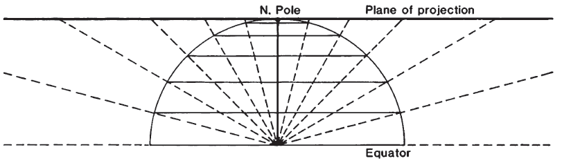
The meridians of the polar Gnomonic projection appear straight, as on other polar azimuthal projections, and parallels of latitude are circles centered about the pole (fig. 34A). The parallels are closest near the pole, and their spacings increase away from the pole much more rapidly than they do on the polar Stereographic. The radii are proportional to the trigonometric tangent of the arc distance from the pole.
On the equatorial aspect, meridians are straight parallel lines perpendicular to the Equator, which is also straight (fig. 34B). The meridians are closest near the central meridian, and the spacing is rapidly increased away from it, the distance from center in proportion to the tangent of the difference in longitude. The parallels other than the Equator are all hyperbolic arcs, symmetrical about the Equator.
Since meridians are great-circle paths, they are also plotted straight on the oblique aspect of the Gnomonic, but they intersect at the pole (fig. 34C). They are not spaced at equal angles. The Equator is a straight line perpendicular to the central meridian. If the central latitude is north of the Equator, its colatitude (90° minus the latitude) is shown as a parabolic arc, more northern latitudes are ellipses, and more southern latitudes are hyperbolas. If the central latitude is south of the Equator, opposite signs apply. FIGURE 34.— Gnomonic projection, range 60° from center. (A) Polar aspect. (B) Equatorial aspect. (C) Oblique aspect, centered at lat. 40° N. All great-circle paths are straight lines on these maps.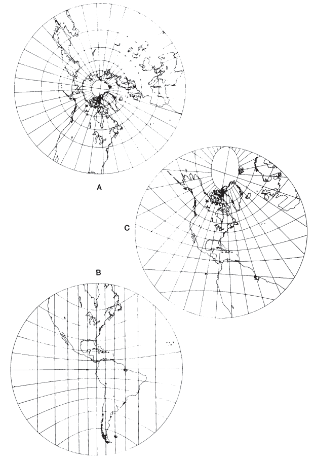
FORMULAS FOR THE SPHERE #
A point at a given angular distance from the chosen center point on the sphere is plotted on the Gnomonic projection at a distance from the center proportional to the trigonometric tangent of that angular distance, and at its true azimuth, or
For the north polar Gnomonic, letting $\phi_1 = 90^\circ$,
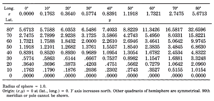
TABLE 26.— Gnomonic projection : Rectangular coordinates for equatorial aspect
23. GENERAL PERSPECTIVE PROJECTION #
SUMMARY #
- Often used to show the Earth or other planets and satellites as seen from space.
- Orthographic, Stereographic, and Gnomonic projections are special forms of the Vertical Perspective.
- Vertical Perspective projections are azimuthal; Tilted Perspectives are not.
- Central meridian and a particular parallel (if shown) are straight lines.
- Other meridians and parallels are usually arcs of circles or ellipses, but some may be parabolas or hyperbolas.
- Neither conformal (unless Stereographic) nor equal-area.
- If the point of perspective is above the sphere or ellipsoid, less than one hemisphere may be shown, unless the view is from infinity (Orthographic). If below center of globe or beyond the far surface, more than one hemisphere may be shown.
- No distortion at the center if a Vertical Perspective is projected onto a tangent plane. Considerable distortion near the projection limit.
- Directions from the center are true on the Vertical Perspective for the sphere and for the polar ellipsoidal form.
- Known by Greeks and Egyptians 2,000 years ago in limiting forms.
HISTORY AND USAGE #
Whenever the Earth is photographed from space, the camera records the view as a perspective projection. If the camera precisely faces the center of the Earth, the projection is Vertical Perspective. Otherwise, a Tilted Perspective projection is obtained. Perspective views have also served other purposes.
With the complication of plotting coordinates for general perspective projections, there was little known interest in them until the 18th century, except for the well-known special cases of the Orthographic, Stereographic, and Gnomonic projections, which are perspective from infinity, the opposite surface, and the center of the sphere, respectively.
In 1701, the French mathematician Philippe De la Hire (1640-1718) found that if the point of perspective is placed 1.71 times the radius of the globe from the center in a direction opposite that of the plane of projection, the Equator on the polar Vertical Perspective projection has exactly twice the radius of the 45th parallel. The other parallels are not quite proportionally spaced, but this represented a use of geometric projection to achieve low distortion. Several other scientists, such as Antoine Parent in 1702 and various mathematicians of the late 19th century, extended this approach to obtain low-distortion projections which meet other criteria.
Of special interest was British geodesist A.R. Clarke’s use of least squares to obtain in 1862 the Vertical Perspective projection with minimum error for the portion of the Earth bounded by a given spherical circle. He determined parameters for several continental areas, and he also presented the “Twilight” projection, with a bounding circle 108" from the center and centered to show much of the land mass of the Earth in one map. All these low- and minimum-error perspective projections were based on “far-side” points of perspective, and they were projected onto a secant plane to reduce overall error (Close and Clarke, 1911, p. 655-656; Snyder, 1985a).
Space exploration beginning in 1957 led to a renewed interest in the perspective projection, although Richard Edes Harrison had used several perspective views in a World War I1 atlas of 1944. Now the concern was for the pictorial view from space, not for minimal distortion. Albert L. Nowicki of the U.S. Army Map Service presented the AMS Lunar Projection, which is a far-side Vertical Perspective based on a perspective center about 1.54 times the radius from the center, to show somewhat more than one hemisphere of the Moon. This recognized the fact that more than half the Moon is seen from the Earth over a period of time. Nowicki called this a “modified Stereographic” projection (Nowicki, 1962). This name has been applied elsewhere to “far-side” Vertical Perspectives, none of which are conformal; it is applied later in this book to complex-algebra modifications of the Stereographic which are conformal but not perspective.
The Tilted Perspective projection is more complicated to compute, but since it has been the projection used in effect for most space photographs, such as those from the manned Gemini and Apollo space missions, it has been analyzed in recent literature.
Weather maps issued by the U.S. National Weather Service have regularly been based on a Vertical Perspective projection as seen from geosynchronous satellites near the Equatorial plane and 42,000 km from the Earth’s center. The USGS has not used the Perspective projection to date for published maps.
FIGURE 35.— Geometric projection of the parallels of the polar Perspective projections, Vertical and Tilted. Distance of point of perspective from center of Earth may be varied, as may the angle of tilt. For ‘far-side’ projection, ‘point of perspective’ would be shown below Equator and usually below South Pole on this drawing.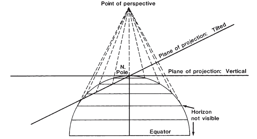
FEATURES #
The general Perspective projection (excepting the three common forms) should be considered primarily as a basis for a view of the Earth from space. The various historical studies described above and leading to low-error azimuthal projections have little practical value, since nonperspective azimuthal projections, like the Azimuthal Equidistant, may be used instead.
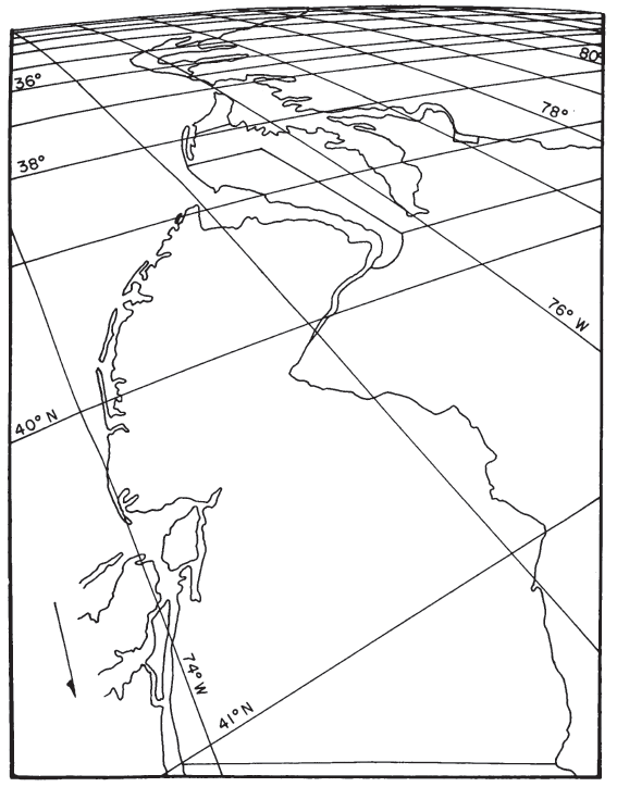
It is therefore of little interest to compute distortion at various locations on the map. There is no distortion at the center of projection with the Vertical Perspective onto a tangent plane (figs. 35 and 36), but there is shape, area, and scale distortion almost everywhere else on perspective maps (except that the Stereographic is conformal). The rapidity with which distortion increases varies with the location of the point of perspective and with the tilt of the plane to the line connecting this point with the center of the Earth (figs. 35 and 37). For the Vertical Perspective, this plane is perpendicular to this line. FIGURE 36.— Vertical Perspective projection. (A) Polar aspect, from 2,000 km above the Earth’s surface. (B) Equatorial aspect, from geosynchronous satellite, 35,800 km above the Earth’s surface. (C) Oblique aspect, centered at lat. 40° N., from 2,000 km above the Earth’s surface FIGURE 37.— Tilted Perspective projection. Eastern seaboard viewed from a point about 160 km above Newburgh, N.Y. 1° graticule.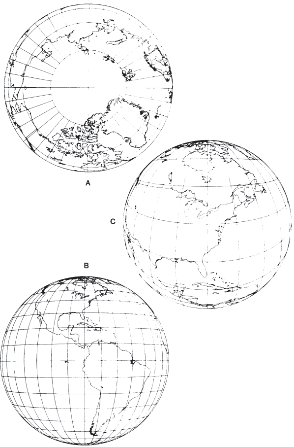
For pictorial and small-scale usage, the spherical equations are adequate. For special large-scale applications, such as Landsat returned-beam-vidicon (RBV) and Space Shuttle Large-Format-Camera images and photographs, the ellipsoidal equations are necessary. The formulas are given below for several possible alternatives.
FORMULAS FOR THE SPHERE #
Vertical Perspective Projection #
A point at a given angular distance $c$ from the center, and at an azimuth $Az$ east of north is plotted in accordance with the following polar coordinates ($\theta$ is measured east of south):
$P$ is the distance of the point of perspective from the center of the Earth, divided by the radius $R$ of the Earth as a sphere. It is positive in the direction of the center of the projection (for the “view from space”) and negative in the opposite direction (for a far-side perspective such as those by Clarke and Nowicki (above), or the Stereographic, for which $P = -1$). In terms of the height $H$ of the point of perspective above the surface, $P = H/R + 1$, or $H = R(P- 1)$. The term $k’$ is the scale factor in a direction perpendicular to the radius from the center of the map, not along the parallel, except in the polar aspect. The scale factor $h’$ is measured in the direction of the radius.
Combining with standard equations, the formulas for rectangular coordinates of the oblique Vertical Perspective projection are as follows, given $R, P, \chi_1, \lambda_0, \phi$, and $\lambda$, to find $x$ and $y$ (see p. 320 for numerical examples):
and $(\phi_1, \lambda_0)$ are latitude and longitude of the projection center and origin. The Y axis coincides with the central meridian $\lambda_0$, $y$ increasing northerly. The map limit is a circle of radius $R[(P-1)/(P+1)]^{1/2}$. Meridians and parallels are generally elliptical arcs, but the central meridian and the latitude whose sine equals $P\sin\phi_1$, are straight lines. For automatic plotting, equation (5-3) should be used to reject points for which $\cos{c}$ is less than $1/P$. These are beyond the range of the map, regardless of whether $P$ is positive or negative.
Because of the number of other equations below, the simplified equations for polar and equatorial aspects are not given here. They may be obtained by entering
the appropriate values of $\phi_1$, in equations (22-4), (22-5), and (5-3). Table 27 shows rectangular coordinates for a hemisphere as seen from a geosynchronous
satellite. TABLE 27.— Vertical Perspective projection: Rectangular coordinates for equatorial aspect from geosynchronous satellite [y coordinate in parentheses under x coordinate]![TABLE 27.— Vertical Perspective projection: Rectangular coordinates for equatorial aspect from geosynchronous satellite [y coordinate in parentheses under x coordinate]](../table27.png)
Tilted Perspective Projection #
The following equations are used in conjunction with the equations above for the Vertical Perspective. While they may be combined, it is easier to follow and more practical to program separately these equations to follow (for forward) or precede (for inverse) those above. For the forward equations, given $R, P, \phi_1, \lambda_0, \omega, \gamma, \phi$, and $\lambda$, $(x,y)$ is first calculated from equations (5-3), (23-3), (22-4), and (22-5) in order, then

FIGURE 38.— Coordinate system for Tilted Perspective projection. The north (N) arrow lies in the vertical plane for the equatorial or oblique aspect. See figure 35 for projection of points onto these planes.
Restated in terms of a camera in space, the camera is placed at a distance $RP$ from the center of the Earth, perpendicularly over point $(\phi_1, \lambda_0)$. The camera is horizontally turned to face $\gamma$ clockwise from north, and then tilted $(90^\circ-\omega)$ downward from horizontal, “horizontal” meaning parallel to a plane tangent to the sphere at $(\phi_1, \lambda_0)$. The photograph is then taken, placing points $(\phi, \lambda)$ in positions $(x_t, y_t)$, based on a scale reduction in $R$. The straight meridian and parallel of the Vertical Perspective are also straight on the Tilted form.
If the tilted plane is perpendicular to the line connecting the point of perspective and the horizon, $\omega = \arcsin (1/P)$. Points for which $\cos{c}$ (equation (5-3)) is less than $(1/P)$ are beyond the map limits, as on the Vertical Perspective, but the map limit is now a conic section of eccentricity equal to $\sin\omega/(1-1/P^2)^{1/2}$. This limit may be plotted by inserting the $(x,y)$ coordinates of the circle representing the Vertical Perspective map limit into equations (23-5) through (23-7) for final plotting coordinates $(x_t, y_t)$, after stating the original equations for the circle in parametric form,
For the inverse equations for the Tilted Perspective projection of the sphere, given$R, P, \phi_1, \lambda_0, \omega,\gamma, x_t$ and $y_t$, first $H$ is calculated from (23-8), and $(x,y)$ are calculated from these equations:
It is also possible to use projective constants $K_1\,-\,K_{11}$ for the sphere as well as the ellipsoid in equations below, but this is not often done for the sphere. If desired, the formulas below may be used for the sphere if the eccentricity is made zero.
FORMULAS FOR THE ELLIPSOID #
Vertical Perspective Projection #
Because of the increased number of equations, they are given in the order of use. Given $a, e^2, P, \phi_1, \lambda_0, h_0, \phi, \lambda$ and $h$, to find $x$ and $y$ (For numerical examples see p. 323):
$P =$ the distance of the point of perspective from the center of the Earth, divided by $a$, the semimajor axis.
$H =$ the height of the point of perspective in a direction perpendicular to the surface of the ellipsoid at nadir point $(\phi_1,\lambda_0)$, but measured from the height $h_0$ of the nadir above the ellipsoid, not above sea level.
$\phi_g =$ the geocentric latitude of the point of perspective, measured as the angle between the direct line from the center to this point, and the equatorial plane, not as the geocentric latitude corresponding to $\phi_1$
$h =$ the height of $(\phi,\lambda)$ above the ellipsoid. The use of $h$ makes these formulas more general, but for most plotting of graticules it would be zero.
If $H$ is given rather than $P$, the latter may be computed as follows:
Since $\phi_g$ is calculated from $P$ in equation (23-17), iteration is involved, with $\phi_1$ as the first trial value of $\phi_g$. The comments following the forward formulas for the sphere apply approximately here. The straight parallel is the latitude $\phi$ whose sine equals $P,a\sin\phi_g/[N(1-e^2)+h]$, if $h$ is a constant, such as zero. This is an iterative calculation with successive substitution of $\phi$, starting with $\phi_1$, as a trial. The central meridian $\lambda_0$, is also straight.
For the inverse formulas for the Vertical Perspective projection of the ellipsoid, given $a, e^2, P, \phi_1, \lambda_0, h_0, h, x$ and $y$, to find $\phi, \lambda$: Equations (23-17) and (23-18) are used to compute $\phi_g$ and $H$ (or (23-21) to compute $P$ if $H$ is given), then
Tilted Perspective Projection Using Projective Equations #
When a photograph or other plane image is obtained from space, projective equations with 11 constants may be used to find the rectangular coordinates of any point of known latitude, longitude, and height above the ellipsoid, in the plane of the image, instead of directly using the orientation of the camera or sensor. The 3-dimensional rectangular coordinates of a point on or off the Earth’s surface can be found from the following equations, taking the semimajor axis $a$ of the Earth as 1.0:
The projective equations are as follows,
The 11 constants $K$, may be determined either from points on the “space photograph” or from the parameters of the “camera.” Although least squares and other corrections are used in determining these constants in analytical photogrammetry for highest precision, the approach given here is confined to the use of measurements which are assumed to the precise. The reader is referred to other texts for the least-squares approach.
To determine $K_1\unicode{x2013}K_{11}$ from six widely spaced identified points on the image, equations (23-41) and (23-42) may be transposed as follows:
To determine $K_1\unicode{x2013}K_{11}$ from parameters of the projection, first $H$ is found from (23-18), then
$(\phi_1, \lambda_0) =$ latitude and longitude of the projection center and origin
$\phi_g =$ geocentric latitude of the point of perspective, found from equation (23-17)
$\gamma=$ azimuth east of north of the Yt axis, or the most upward-tilted axis of the plane of projection
$\omega =$ upward angle of tilt
$P =$ distance from the center of the Earth to the point of perspective, divided by $a$, the semimajor axis.
New symbols are as follows:
$\theta =$ clockwise angle through which the (Xt, Yt) axes are rotated for the arbitrary axes (X’t, Y’t) used for the constants $K_1\unicode{x2013}K_{11}$. This may be made zero to retain the (Xt, Yt) axes.
$(x_0, y_0) =$ offsets of the (Xt, Yt) axes to establish a different origin for the (X’t, Y’t) axes. They may also be set at zero to retain the (Xt, Yt) axes.
The two sets of axes are related as follows:
For inverse computations using projective constants given $K_1\unicode{x2013}K_{11}, x’_t$ and $y’_t$, to find $\phi$ and $\lambda$, the following are calculated in order:
where $E$ is found from (23-36) if $h$ is not zero, or $E = 1$ if $h$ is zero. Then
and $\phi$ is found from (23-35) if $h$ is not zero, or (23-37) if $h$ is zero, taking one sign in (23-79) for the latitude desired, and the opposite sign for the latitude hidden from view at the same coordinates. The same sign applies throughout the map, once it is determined for a point for which the latitude is obviously right or wrong.
If $h$ is not zero, $E$ is initially assumed to be 1. After trial values of $\phi$ and $\lambda$ are determined above, an $h$ suitable for that point may be used with the new $\phi$ in calculating $E$; then $A_{16}, S, \phi$ and $\lambda$ are recalculated. Iteration continues until the change in the calculated $\phi$ is negligible.
If $h$ is zero, since $E = 1$ and (23-37) is explicit in $\phi$, no iteration is required.
Finally, to compute “camera” parameters from given constants $K_1\unicode{x2013}K_{11}$ (Bender, ca. 1970, p. 26-27), given $a, e^2$, and an assumed $h_0$, first the following three simultaneous equations are solved for $X_0, Y_0,$ and $Z_0$, the space coordinates of the point of perspective divided by $a$ (see description of axes following (23-40)):
24. LAMBERT AZIMUTHAL EQUAL-AREA PROJECTION #
SUMMARY #
- Azimuthal.
- Equal-Area.
- All meridians in the polar aspect, the central meridian in other aspects, and the Equator in the equatorial aspect are straight lines.
- The outer meridian of a hemisphere in the equatorial aspect (for the sphere) and the parallels in the polar aspect (sphere or ellipsoid) are circles.
- All other meridians and parallels are complex curves.
- Not a perspective projection.
- Scale decreases radially as the distance increases from the center, the only point without distortion.
- Scale increases in the direction perpendicular to radii as the distance increases from the center.
- Directions from the center are true for the sphere and the polar ellipsoidal forms.
- Point opposite the center is shown as a circle surrounding the map (for the sphere).
- Used for maps of continents and hemispheres.
- Presented by Lambert in 1772.
HISTORY #
The last major projection presented by Johann Heinrich Lambert in his 1772 Beiträge was his azimuthal equal-area projection (Lambert, 1772, p. 75-78). His name is usually applied to the projection in modem references, but it is occasionally called merely the Azimuthal (or Zenithal) Equal-Area projection. Not only is it equal-area, with, of course, the azimuthal property showing true directions from the center of the projection, but its scale at a given distance from the center varies less from the scale at the center than the scale of any of the other major azimuthals (see table 21).
Lambert discussed the polar and equatorial aspects of the Azimuthal Equal-Area projection, but the oblique aspect is just as popular now. The polar aspect was apparently independently derived by Lorgna in Italy in 1789, and the latter was called the originator in a publication a century later (USC&GS, 1882, p. 290). G. A. Ginzburg proposed two modifications of the general Lambert Azimuthal projection in 1949 to reduce the angular distortion at the expense of creating a slight distortion in area (Maling, 1960, p. 206). A common modification was devised by Ernst Hammer in 1892 and is called the Hammer or Hammer-Aitoff projection. It consists of halving the vertical coordinates of the equatorial aspect of one hemisphere and doubling the values of the meridians from center. It retains equality of area, but it is no longer azimuthal.
FEATURES #
The Lambert Azimuthal Equal-Area projection is not a perspective projection. It may be called a “synthetic” azimuthal in that it was derived for the specific purpose of maintaining equal area. The ellipsoidal form maintains equal area, but it is not quite azimuthal except in the polar aspect, so the name for the general ellipsoidal form is a slight misnomer, although it looks like the spherical azimuthal form and has most of its other characteristics.
The polar aspect (fig. 39A), like that of the Orthographic and Stereographic, has circles for parallels of latitude, all centered about the North or South Pole, and straight equally spaced radii of these circles for meridians. The difference is, once again, in the spacing of the parallels. For the Lambert, the spacing between the parallels gradually decreases with increasing distance from the pole. The opposite pole, not visible on either the Orthographic or Stereographic, may be shown on the Lambert as a large circle surrounding the map, almost half again as far as the Equator from the center. Normally, the projection is not shown beyond one hemisphere (or beyond the Equator in the polar aspect).
The equatorial aspect (fig. 39B) has, like the other azimuthals, a straight Equator and straight central meridian, with a circle representing the 90th meridian east and west of the central meridian. Unlike those for the Orthographic and Stereographic, the remaining meridians and parallels are uncommon complex curves. The chief visual distinguishing characteristic is that the spacing of the meridians near the 90th meridian and sf the parallels near the poles is about 0.7 of the spacing at the center of the projection, or moderately less to the eye. The parallels of latitude look considerably like circular arcs, except near the 90th meridians, where they exhibit a noticeable turn toward the nearest pole.
The oblique aspect (fig. 39C) of the Lambert Azimuthal Equal-Area resembles the Orthographic to some extent, until it is seen that crowding is far less pronounced as the distance from the center increases. Aside from the straight central meridian, all meridians and parallels are complex curves, not ellipses.
In both the equatorial and oblique aspects, the point opposite the center may be shown as a circle surrounding the map, corresponding to the opposite pole in the polar aspect. Except for the advantage of showing the entire Earth in an equal-area projection from one point, the distortion is so great beyond the inner hemisphere that for world maps the Earth should be shown as two separate hemispherical maps, the second map centered on the point opposite the center of the first map. FIGURE 39.— Lambert Azimuthal Equal-Area projection. (A) Polar aspect showing one hemisphere; the entire globe may be included in a circle of 1.41 times the diameter of the Equator. (B) Equatorial aspect; frequently used in atlases for maps of the Eastern and Western hemispheres. (C) Oblique aspect; centered on lat. 40° N.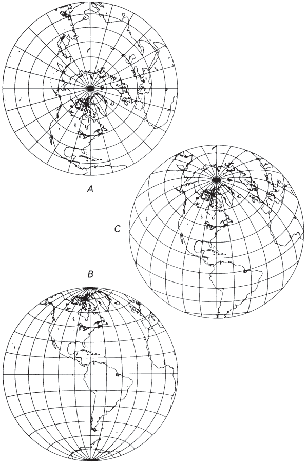
USAGE #
The spherical form in all three aspects of the Lambert Azimuthal Equal-Area projection has appeared in recent commercial atlases for Eastern and Western Hemispheres (replacing the long-used Globular projection) and for maps of oceans and most of the continents and polar regions.
The polar aspect appears in the National Atlas (USGS, 1970, p. 148-149) for maps delineating north and south polar expeditions, at a scale of 1:39,000,000. It is used at a scale of 1:20,000,000 for the Arctic Region as an inset on the 1978 USGS Map of Prospective Hydrocarbon Provinces of the World.
The USGS has prepared six base maps of the Pacific Ocean on the spherical form of the Lambert Azimuthal Equal-Area. Four sections, at 1:10,000,000, have centers at 35° N., 150° E. ; 35° N., 135° W.; 35° S., 135° E.; and 40° S., 100° W. The Pacific-Antarctic region, at a scale of 1:8,300,000, is centered at 20° S. and 165° W., while a Pacific Basin map at 1:17,100,000 is centered at the Equator and 160° W. (The last two maps were originally erroneously labeled with scales that are too small.) The base maps have been used for individual geographic, geologic, tectonic, minerals, and energy maps. The USGS has also cooperated with the National Geographic Society in revising maps of the entire Moon drawn to the spherical form of the equatorial Lambert Azimuthal Equal-Area.
GEOMETRIC CONSTRUCTION #
The polar aspect (for the sphere) may be drawn with a simple geometric construction: In figure 40, if angle AOR is the latitude $\phi$ and P is the pole at the center, PA is the radius of that latitude on the polar map. The oblique and equatorial aspects have no direct geometric construction. They may be prepared indirectly by using other azimuthal projections (Harrison, 1943), but it is now simpler to plot automatically or manually from rectangular coordinates which are generated by a relatively simple computer program. The formulas are given below. FIGURE 40.— Geometric construction of polar Lambert Azimuthal Equal-Area projection.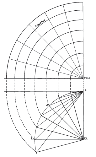
FORMULAS FOR THE SPHERE #
On the Lambert Azimuthal Equal-Area projection for the sphere, a point at a given angular distance from the center of projection is plotted at a distance from the center proportional to the sine of half that angular distance, and at its true azimuth, or
For the north polar Lambert Azimuthal Equal-Area, with $\phi_1=90^\circ$, since $k’$ is $k$ for the polar aspect, these formulas simplify to the following (see numerical examples):
If $\rho = 0$, equations (20-14) through (20-17) are indeterminate, but $\phi = \phi_1$, and $\lambda = \lambda_0$. If $\phi_1$ is not $\pm90°$,
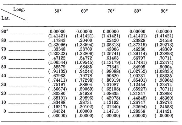
Table 28 lists rectangular coordinates for the equatorial aspect for a 10° graticule with a sphere of radius $R = 1.0$. TABLE 28.— Lambert Azimuthal Equal-Area projection: Rectangular coordinates for equatorial aspect (sphere)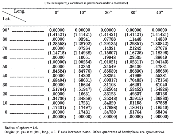
FORMULAS FOR THE ELLIPSOID #
As noted above, the ellipsoidal oblique aspect of the Lambert Azimuthal Equal-Area projection is slightly nonazimuthal in order to preserve equality of area. To date, the USGS has not used the ellipsoidal form in any aspect. The formulas are analogous to the spherical equations, but involve replacing the geodetic latitude $\phi$ with authalic latitude $\beta$ (see equation (3-11)). In order to achieve correct scale in all directions at the center of projection, that is, to make the center a “standard point,” a slight adjustment using $D$ is also necessary. The general forward formulas for the oblique aspect are as follows, given $a, e, \phi_1, \lambda_0, \phi,$ and $\lambda$ (see numerical examples):
For the south polar aspect, $(\phi_1 = -90^\circ)$, equations (21-30) and (21-32) remain the same, but
The inverse formulas for the polar aspects involve relatively simple transformations of above equations (21-30), (21-31), and (24-23), except that $\phi$ is found from the iterative equation (3-16), listed just above, in which $q$ is calculated as follows:
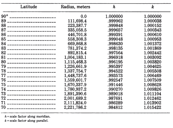
TABLE 29.— Ellipsoidal polar Lambert Azimuthal Equal-Area projection (International ellipsoid)
25. AZIMUTHAL EQUIDISTANT PROJECTION #
SUMMARY #
- Azimuthal.
- Distances measured from the center are true.
- Distances not measured along radii from the center are not correct.
- The center of projection is the only point without distortion.
- Directions from the center are true (except on some oblique and equatorial ellipsoidal forms).
- Neither equal-area nor conformal.
- All meridians on the polar aspect, the central meridian on other aspects, and the Equator on the equatorial aspect are straight lines.
- Parallels on the polar projection are circles spaced at true intervals (equidistant for the sphere).
- The outer meridian of a hemisphere on the equatorial aspect (for the sphere) is a circle.
- All other meridians and parallels are complex curves.
- Not a perspective projection.
- Point opposite the center is shown as a circle (for the sphere) surrounding the map.
- Used in the polar aspect for world maps and maps of polar hemispheres.
- Used in the oblique aspect for atlas maps of continents and world maps for aviation and radio use.
- Known for many centuries in the polar aspect.
HISTORY #
While the Orthographic is probably the most familiar azimuthal projection, the Azimuthal Equidistant, especially in its polar form, has found its way into many atlases with the coming of the air age for maps of the Northern and Southern Hemispheres or for world maps. The simplicity of the polar aspect for the sphere, with equally spaced meridians and equidistant concentric circles for parallels of latitude, has made it easier to understand than most other projections. The primary feature, showing distances and directions correctly from one point on the Earth’s surface, is also easily accepted. In addition, its linear scale distortion is moderate and falls between that of equal-area and conformal projections.
Like the Orthographic, Stereographic, and Gnomonic projections, the Azimuthal Equidistant was apparently used centuries before the 15th-century surge in scientific mapmaking. It is believed that Egyptians used the polar aspect for star charts, but the oldest existing celestial map on the projection was prepared in 1426 by Conrad of Dyffenbach. It was also used in principle for small areas by mariners from earliest times in order to chart coasts, using distances and directions obtained at sea.
The first clear examples of the use of the Azimuthal Equidistant for polar maps of the Earth are those included by Gerardus Mercator as insets on his 1569 world map, which introduced his famous cylindrical projection. As Northern and Southern Hemispheres, the projection appeared in a manuscript of about 1510 by the Swiss Henricus Loritus, usually called Glareanus (1488-1563), and by several others in the next few decades (Keuning, 1955, p. 4-5). Guillaume Postel is given credit in France for its origin, although he did not use it until 1581. Antonio Cagnoli even gave the projection his name as originator in 1799 (Deetz and Adams, 1934, p. 163; Steers, 1970, p. 234). Philippe Hatt developed ellipsoidal versions of the oblique aspect which are used by the French and the Greeks for coastal or topographic mapping.
Two projections with similar names are called the Two-Point Azimuthal and the Two-Point Equidistant projections. Both were developed about 1920 independently by Maurer (1919) of Germany and Close (1921) of England. The first projection (rarely used) is geometrically a tilting of the Gnomonic projection to provide true azimuths from either of two chosen points instead of from just one. Like the Gnomonic; it shows all great circle arcs as straight lines and is limited to one hemisphere. The Two-Point Equidistant has received moderate use and interest, and shows true distances, but not true azimuths, from either of two chosen points to any other point on the map, which may be extended to show the entire world (Close, 1934).
The Chamberlin Trimetric projection is an approximate “three-point equidistant” projection, constructed so that distances from three chosen points to any other point on the map are approximately correct. The latter distances cannot be exactly true, but the projection is a compromise which the National Geographic Society uses as a standard projection for maps of most continents. This projection was geometrically constructed by the Society, of which Wellman Chamberlin (1908-76) was chief cartographer for many years.
An ellipsoidal adaptation of the Two-Point Equidistant was made by Jay K. Donald of American Telephone and Telegraph Company in 1956 to develop a grid still used by the Bell Telephone system for establishing the distance component of long distance rates. Still another approach is Bomford’s modification of the Azimuthal Equidistant, in which the usual circles of constant scale factor perpendicular to the radius from the center are made ovals to give a better average scale factor on a map with a rectangular border (Lewis and Campbell, 1951, p. 7, 12-15).
FEATURES #
The Azimuthal Equidistant projection, like the Lambert Azimuthal Equal-Area, is not a perspective projection, but in the spherical form, and in some of the ellipsoidal forms, it has the azimuthal characteristic that all directions or azimuths are correct when measured from the center of the projection. As its special feature, all distances are at true scale when measured between this center and any other point on the map.
The polar aspect (fig. 41A), like other polar azimuthals, has circles for parallels of latitude, all centered about the North or South Pole, and equally spaced radii of these circles for meridians. The parallels are, however, spaced equidistantly on the spherical form (or according to actual parallel spacings on the ellipsoid). A world map can extend to the opposite pole, but distortion becomes infinite. Even though the map is finite, the point for the opposite pole is shown as a circle twice the radius of the mapped Equator, thus giving an infinite scale factor along that circle. Likewise, the countries of the outer hemisphere are visibly increasingly distorted as the distance from the center increases, while the inner hemisphere has little enough distortion to appear rather satisfactory to the eye, although the east-west scale along the Equator is almost 60 percent greater than the scale at the center.
As on other azimuthals, there is no distortion at the center of the projection and, as on azimuthals other than the Stereographic, the scale cannot be reduced at the center to provide a standard circle of no distortion elsewhere. It is possible to use an average scale over the map involved to minimize variations in scale error in any direction, but this defeats the main purpose of the projection, that of providing true distance from the center. Therefore, the scale at the projection center should be used for any Azimuthal Equidistant map.
The equatorial aspect (fig. 41B) is least used of the three Azimuthal Equidistant aspects, primarily because there are no cities along the Equator from which distances in all directions have been of much interest to map users. Its potential use as a map of the Eastern or Western Hemisphere was usually supplanted first by the equatorial Stereographic projection, later by the Globular projection (both graticules drawn entirely with arcs of circles and straight lines), and now by the equatorial Lambert Azimuthal Equal-Area.
For the equatorial Azimuthal Equidistant projection of the sphere, the only straight lines are the central meridian and the Equator. The outer circle for one hemisphere (the meridian 90" east and west of the central meridian) is equidistantly marked off for the parallels, as it is on other azimuthals. The other meridians and parallels are complex curves constructed to maintain the correct distances and azimuths from the center. The parallels cross the central meridian at their true equidistant spacings, and the meridians cross the Equator equidistantly. The map can be extended, like the polar aspect, to include a much-distorted second hemisphere on the same center.
The oblique Azimuthal Equidistant projection (fig. 41C) rather resembles the oblique Lambert Azimuthal Equal-Area when confined to the inner hemisphere centered on any chosen point between Equator and pole. Except for the straight central meridian, the graticule consists of complex curves, positioned to maintain true distance and azimuth from the center. When the outer hemisphere is included, the difference between the Equidistant and the Lambert becomes more pronounced, and while distortion is as extreme as in other aspects, the distances and directions of the features from the center now outweigh the distortion for many applications. FIGURE 41.— Azimuthal Equidistant projection. (A) Polar aspect extending to the South Pole; commonly used in atlases for polar maps. (B) Equatorial aspect. (C) Oblique aspect centered on lat. 40° N. Distance from the center is true to scale.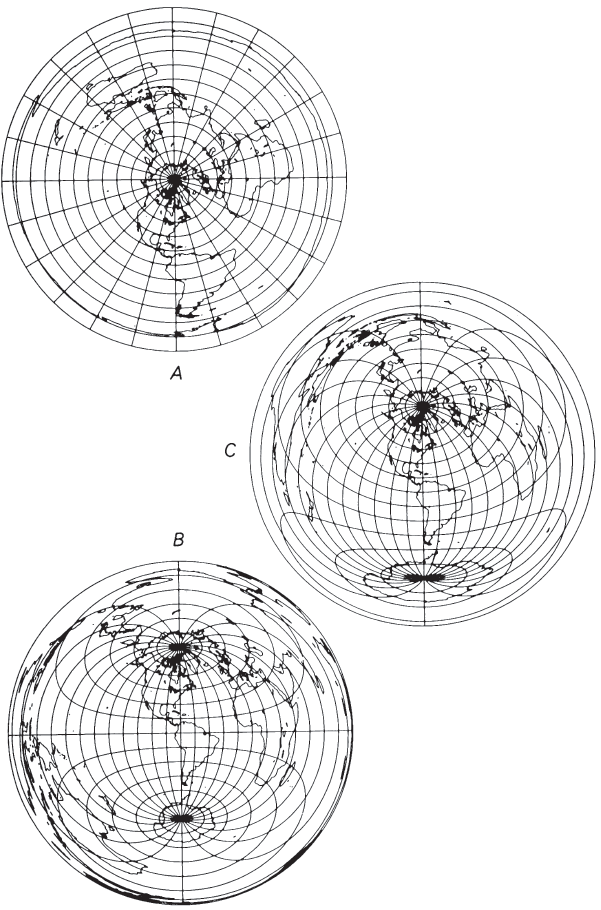
USAGE #
The polar aspect of the Azimuthal Equidistant has regularly appeared in commercial atlases issued during the past century as the most common projection for maps of the north and south polar areas. It is used for polar insets on Van der Grinten-projection world maps published by the National Geographic Society and used as base maps (including the insets) by USGS. The polar Azimuthal Equidistant projection is also normally used when a hemisphere or complete sphere centered on the North or South Pole is to be shown. The oblique aspect has been used for maps of the world centered on important cities or sites and occasionally for maps of continents. Nearly all these maps use the spherical form of the projection.
The USGS has used the Azimuthal Equidistant projection in both spherical and ellipsoidal form. An oblique spherical version of the Earth centered at lat. 40° N., long. 100° W., appears in the National Atlas (USGS, 1970, p. 329). At a scale of 1:175,000,000, it does not show meridians and parallels, but shows circles at 1,000-mile intervals from the center. The ellipsoidal oblique aspect is used for the plane coordinate projection system in approximate form for Guam and in nearly rigorous form for islands in Micronesia.
GEOMETRIC CONSTRUCTION #
The polar Azimuthal Equidistant is among the easiest projections to construct geometrically, since the parallels of latitude are equally spaced in the spherical case and the meridians are drawn at their true angles. There are no direct geometric constructions for the oblique and equatorial aspects. Like the Lambert Azimuthal Equal-Area, they may be prepared indirectly by using other azimuthal projections (Harrison, 1943), but automatic computer plotting or manual plotting of calculated rectangular coordinates is the most suitable means now available.
FORMULAS FOR THE SPHERE #
On the Azimuthal Equidistant projection for the sphere, a given point is plotted at a distance from the center of the map proportional to the distance on the sphere and at its true azimuth, or
For the north polar aspect, with $\phi_1 = 90^\circ$,
Table 30 shows rectangular coordinates for the equatorial aspect for a 10° graticule with a sphere of radius $R = 1.0$. TABLE 30.— Azimuthal Equidistant projection: Rectangular coordinates for equatorial aspect (sphere)

FORMULAS FOR THE ELLIPSOID #
The formulas for the polar aspect of the ellipsoidal Azimuthal Equidistant projection are relatively simple and are theoretically accurate for a map of the entire world. However, such a use is unnecessary because the errors of the sphere versus the ellipsoid become insignificant when compared to the basic errors of projection. The polar form is truly azimuthal as well as equidistant. Given $a, e, \lambda_0, \phi_1, \phi,$ and $\lambda$, for the north polar aspect, $\phi_1 = 90^\circ$ (numerical examples):
Table 31 lists polar coordinates for the ellipsoidal aspect of the Azimuthal Equidistant, using the International ellipsoid. TABLE 31.— Ellipsoidal Azimuthal Equidistant projection (International ellipsoid)—Polar Aspect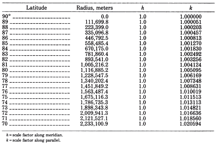
For the oblique and equatorial aspects of the ellipsoidal Azimuthal Equidistant, both nearly rigorous and approximate sets of formulas have been derived. For mapping of Guam, the National Geodetic Survey and the USGS use an approximation to the ellipsoidal oblique Azimuthal Equidistant called the “Guam projection.” It is described by Claire (1968, p. 52-53) as follows (changing his symbols to match those in this publication):
The plane coordinates of the geodetic stations on Guam were obtained by first computing the geodetic distances [$c$] and azimuths [$Az$] of all points from the origin by inverse computations. The coordinates were then computed by the equations: [$x = c \sin {Az}$ and $y = c \cos {Az}$]. This really gives a true azimuthal equidistant projection. The equations given here are simpler, however, than those for a geodetic inverse computation, and the resulting coordinates computed using them will not be significantly different from those computed rigidly by inverse computation. This is the reason it is called an approximate azimuthal equidistant projection.
The formulas for the Guam projection are equivalent to the following:
For Guam, $\phi_1 = 13^\circ28'20.87887’’$ N. lat. and $\lambda_0 = 144^\circ44'55.50254’’$ E. long., with 50,000 m added to both $x$ and $y$ to eliminate negative numbers. The Clarke 1866 ellipsoid is used. The above formulas provide coordinates within 5 mm at full scale of those using ellipsoidal Polyconic formulas for the region of Guam.
A more complicated and more accurate approach to the oblique ellipsoidal Azimuthal Equidistant projection is used for plane coordinates of various individual islands of Micronesia. In this form, the true distance and azimuth of any point on the island or in nearby waters are measured from the origin chosen for the island and along the normal section or plane containing the perpendicular to the surface of the ellipsoid at the origin. This is not exactly the same as the shortest or geodesic distance between the points, but the difference is negligible (Bomford, 1971, p. 125). This distance and azimuth are plotted on the map. The projection is, therefore, equidistant and azimuthal with respect to the center and appears to satisfy all the requirements for an ellipsoidal Azimuthal Equidistant projection, although it is described as a “modified” form. The origin is assigned large-enough values of x and y to prevent negative readings.
The formulas for calculation of this distance and azimuth have been published in various forms, depending on the maximum distance involved. The projection system for Micronesia makes use of “Clarke’s best formula” and Robbins’ inverse of this. These are considered suitable for lines up to 800 km in length. The formulas below, rearranged slightly from Robbins’ formulas as given in Bomford (1971, p. 136-137), are extended to produce rectangular coordinates. No iteration is required. They are listed in the order of use, given a central point at lat. $\phi_1$, long. $\lambda_0$, coordinates $x_0$ and $y_0$ of the central point, the Y axis along the central meridian $\lambda_0$, y increasing northerly, ellipsoidal parameters $a$ and $e$, and $\phi$ and $\lambda$.
Table 32 shows the parameters for the various islands mapped with this projection. TABLE 32.— Plane coordinate systems for Micronesia: Clarke 1866 ellipsoid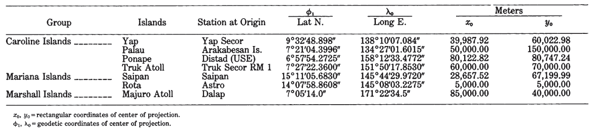
For the Micronesia version of the ellipsoidal Azimuthal Equidistant projection, the inverse formulas given below are “Clarke’s best formula,” as given in Bomford (1971, p. 133) and do not involve iteration. They have also been rearranged to begin with rectangular coordinates, but they are also suitable for finding latitude and longitude accurately for a point at any given distance $c$ (up to about 800 km) and azimuth $Az$ (east of north) from the center, if equations (25-32) and (25-33) are deleted. In order of use, given $a, e$, central point at lat. $\phi_1$, long. $\lambda_0$, rectangular coordinates of center $x_0, y_0$, and $x$ and $y$ for another point, to find $\phi$ and $\lambda$:
To convert coordinates measured on an existing Azimuthal Equidistant map (or other azimuthal map projection), the user may choose any meridian for $\lambda_0$ on the polar aspect, but only the original meridian and parallel may be used for $\lambda_0$ and $\phi_1$ respectively, on other aspects.
26. MODIFIED-STEREOGRAPHIC CONFORMAL PROJECTIONS #
SUMMARY #
- Modified azimuthal.
- Conformal.
- All meridians and parallels are normally complex curves, although some may be straight under some conditions.
- Scale is true along irregular lines, but map is usually designed to minimize scale variation throughout a selected region.
- Map is normally not symmetrical about any axis or point.
- Used for maps of continents in the Eastern Hemisphere, for the Pacific Ocean, and for maps of Alaska and the 50 United States.
- Specific forms devised by Miller, Lee, and Snyder, 1950-84.
HISTORY AND USAGE #
Two short mathematical formulas, taken as a pair, absolutely define the conformal transformation of one surface onto another surface. These formulas are called the Cauchy-Riemann equations, after two 19th-century mathematicians who added rigorous analysis to principles developed in the middle of the 18th century by physicist D’Alembert. Much later, Driencourt and Laborde (1932, vol. 14, p. 242) presented a fairly simple series (equation (26-4) below without the R), involving complex algebra (with imaginary numbers), that fully satisfies the Cauchy-Riemann equations and permits the formation of an endless number of new conformal map projections when certain constants are changed.
The advantage of this series is that lines of constant scale may be made to follow one of a variety of patterns, instead of following the great or small circles of the common conformal projections. The disadvantage is that the length of the series and the computations become increasingly lengthy as the irregularity of the lines of constant scale increases, but this problem has decreased with the development of computers.
Laborde (1928; Reignier, 1957, p. 130) applied this transformation to the mapping of Madagascar, starting with the Oblique Mercator projection and applying the complex equation up to the third-order or cubic terms. Miller (1953) used the same order of complex equation, but began with an oblique Stereographic projection. His resulting map of Europe and Africa has oval lines of constant scale (fig. 42); this projection is called the Miller Oblated (or Prolated) Stereographic. He subsequently (Miller, 1955) prepared similar projections for Asia and Australia each precisely conformal, but he linked them with nonconformal “fill-in” projections to provide a continuous map (in several sheets) of the land masses of the Eastern Hemisphere.
FIGURE 42.— Miller Oblated Stereographic projection of Europe and Africa, showing oval lines of constant scale. Center of projection lat. 18° N., long. 20° E.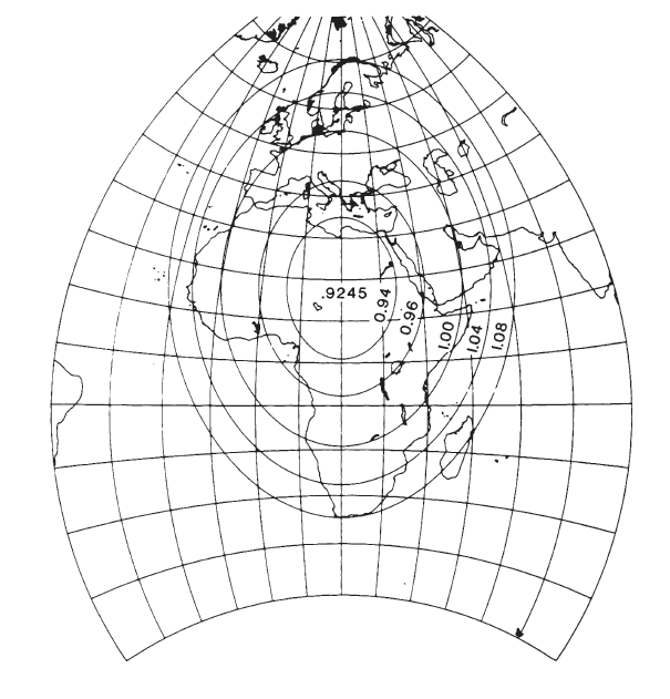
Lee (1974) designed a map of the Pacific Ocean, also using an oblique Stereographic with a third-order complex polynomial. The third-order polynomials used by Laborde, Miller, and Lee make relatively moderate computational demands, because several of the coefficients are zero, and the complex algebra can be readily simplified to equations without imaginary numbers. Recently Reilly (1973) and the writer (Snyder, 1984a, 1985a) have used much higher-order complex equations, but modern computers can readily handle them. Reilly used sixth-order coefficients with the regular Mercator for the new official New Zealand Map Grid, while the writer, beginning with oblique Stereographic projections, used sixth-order coefficients for a map of Alaska and tenth-order for a map of the 50 United States (figs. 43, 44). For these sixth- and tenth-order equations, only one coefficient is zero, but the other coefficients were computed using least squares. The projection for Alaska was used in 1985 by Alvaro F. Espinosa of the USGS to depict earthquake information for that State. The “Modified Transverse Mercator” projection is still being used by the USGS for most maps of Alaska.
FIGURE 43.— GS50 projection, with lines of constant scale factor superimposed. All 50 States, including islands and passages between Alaska, Hawaii, and the conterminous 48 States are shown with scale factors ranging only from 1.02 to 0.98.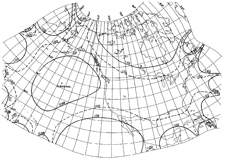
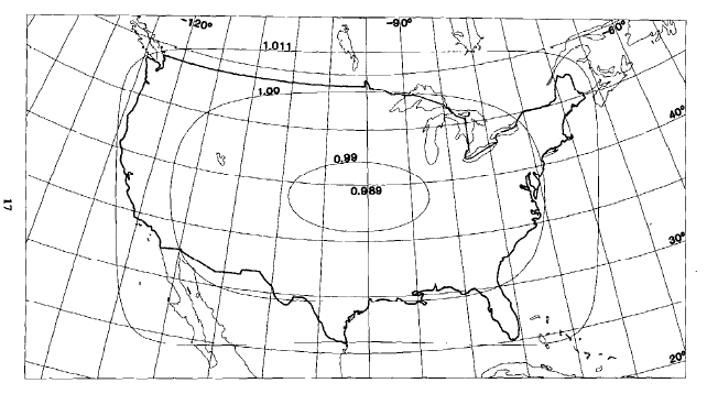
FIGURE 44.— Modified-Stereographic Conformal projection of Alaska, with lines of constant scale superimposed. Scale factors for Alaska range from 0.997 to 1.003, one-fourth the range for a corresponding conic projection. FIGURE 45.— Modified-Stereographic Conformal projection of 48 United States, bounded by a near-rectangle of constant scale. Three lines of constant scale are superimposed. Region bounded by near-rectangle has minimum error.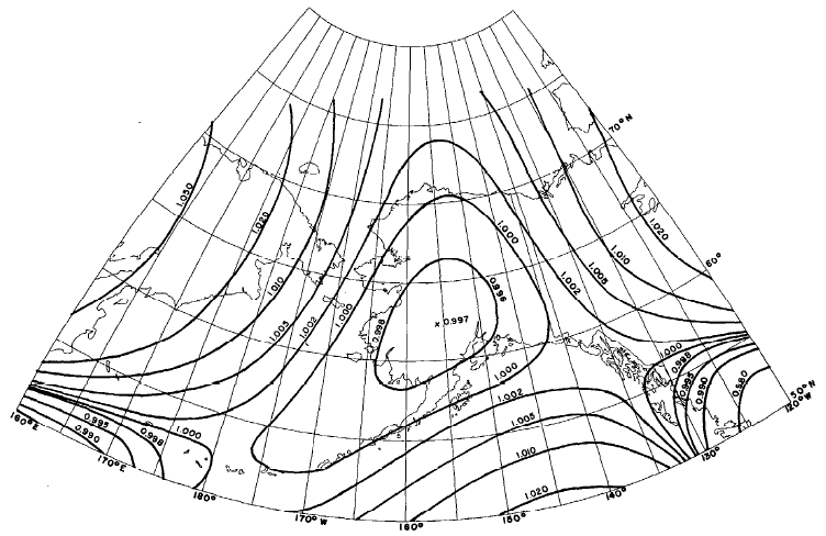
FEATURES #
The common feature linking the endless possibilities of map projections discussed in this chapter is the fact that they are perfectly conformal regardless of the order of the complex-algebra transformation, and regardless of the initial projection, provided it is also conformal.
Chebyshev (1856) stated that a region may be best shown conformally if the sum of the squares of the scale errors (scale factors minus 1) over the region is a minimum. He further declared that this results if the region is bounded by a line of constant scale. This was proven later. Thus the Stereographic is suitable for regions approximately circular in shape, but regions bounded by ovals, regular polygons, or rectangles may be mapped with nearly minimum error by suitably altering the Stereographic with the complex-algebra transformation.
If the region is irregular, such as Alaska, the region of interest may be divided into small elements, and the coefficients may be calculated using least squares to minimize the scale variation for the region shown. The resulting coefficients for the selected projections are given below, but the formulas for least-squares summation are not included here because they are lengthy and are only needed to devise new projections. For them the reader may refer to Snyder (1984a, 198413, 1985a).
The reduction of scale variation by using this complex-algebra transformation makes the ellipsoidal form even more important. This form is also simpler in these cases than for the Transverse Mercator and some other projections, because the lines of true scale normally do not follow a selected meridian, parallel, or other easily identifiable line in any case. Therefore, use of the conformal latitude in place of the geographic latitude is sufficient for the ellipsoidal form. This merely slightly shifts the lines of constant scale from one set of arbitrary locations to another. The coefficients have somewhat different values, however.
The meridians and parallels of the Modified-Stereographic projections are generally curved, and there is usually no symmetry about any point or line. There are limitations to these transformations. Most of them can only be used within a limited range, depending on the number and values of coefficients. As the distance from the projection center increases, the meridians, parallels, and shorelines begin to exhibit loops, overlapping, and other undesirable curves. A world map using the GS50 (50-State) projection is almost illegible, with meridians and parallels intertwined like wild vines.
Within the intended range of the map, the Modified-Stereographic projections can reduce the range of scale variation considerably when compared with standard conformal projections. The tenth-order complex-algebra modification used for the 50-State projection has a scale range of only ±2 percent (or 4 percent overall) for all 50 States placed in their relative geographical positions, including all islands, adjacent waters, water channels connecting Alaska, Hawaii, and the other 48 States, and nearby Canada and Mexico (fig. 43). A Lambert Conformal Conic projection previously used with standard parallels 37° and 65° N. to show the 50 States has a scale range of + 12 to -3 percent (or 15 percent overall). The sixth-order modification for the Alaska map, called the Modified-Stereographic Conformal projection, has a range of ±0.3 percent (or 0.6 percent overall) for Alaska itself, while a Lambert Conformal Conic with standard parallels 55° and 65° N. ranges from + 2.0 to -0.4 percent, or 2.4 percent overall.
The bounding of regions by ovals, near-regular polygons, or near-rectangles of constant scale results in improvement of scale variation by amounts depending on the size and shape of the boundary. The improvement in mean scale error is about 15 to 20 percent using a near-square instead of the circle of the base Stereographic projection. Using a Modified-Stereographic bounded by a near-rectangle instead of an oblique Mercator projection provides a mean improvement of up to 30 percent in some cases, but only 5 to 10 percent in cases involving a long narrow region. For fig. 45, the range of scale is ±1.1 percent (or 2.2 percent overall) within the 48 States, while the Lambert Conformal Conic normally used has a range of +2.4 to -0.6 percent (or 3.0 percent overall).
The improvement for the region in question is made at the expense of scale preservation outside the region. The regular conic projections maintain the same scale range around the entire world between the same latitude limits, even though most of that region is not shown on the regional maps described above.
FORMULAS FOR THE SPHERE #
The Modified-Stereographic conformal projections which have a scale range of more than 5 percent, such as regions bounded by rectangles 80° by 40° in spherical degrees, may satisfactorily be computed for the sphere instead of the ellipsoid. As stated above, development of coefficients is not shown here. For the calculation of final rectangular coordinates, given $R, \phi_1, \lambda_0, A_1$ through $A_m, B_1$ through $B_m$, $\phi,$ and $\lambda$, and to find $x$ and $y$ (see numerical examples):
For the practical computation of equations (26-4) and (26-5), Knuth’s (1969) algorithm is recommended instead of them. LetNote1
For inverse equations, given $R, \phi_1, \lambda_0, A_1$ through $A_m, B_1$ through $B_m$, $x$, and $y$, to find $\phi$ and $\lambda$, first a Newton-Raphson iteration may be used as follows to find $(x’ , y’)$:
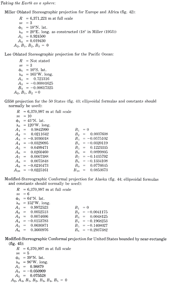
TABLE 33.— Modified-Stereographic Conformal projections: Coefficients for specific forms
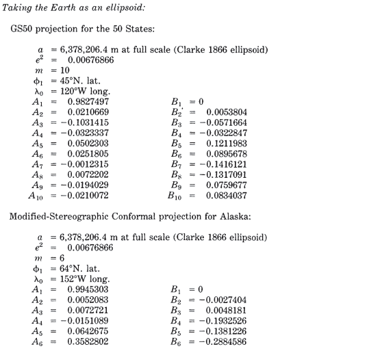
TABLE 33.— Modified-Stereographic Conformal projections: Coefficients for specific forms (Continued)
FORMULAS FOR THE ELLIPSOID #
For higher precision maps taking greater advantage of the reduced scale variation available with Modified-Stereographic Conformal projections, the ellipsoidal formulas should be used. Given $a, e, \phi_1, \lambda_0, A_1$ through $A_m, B_1$ through $B_m, \phi,$ and $\lambda$, to find $x$ and $y$ (special numerical examples are not given, but examples of the ellipsoidal Stereographic, and of the spherical Modified-Stereographic p. 344, are sufficiently similar):
For inverse equations, given $a, e, \phi_1,\lambda_0, A_1$ through $A_m, B_1$ through $B_m, x$, and $y$, to find $\phi$ and $\lambda$, the Newton-Raphson iteration of spherical equations (26-10) through (26-13) is used unchanged to find $(x’, y’)$ except that $R$ is replaced with $a$, and ellipsoidal constants must be used. After convergence, the final $(x’, y’)$ is converted to $(\phi$, \lambda)$ without iteration. Equations (26-14), (26-15), and (3-1) are used to calculate $\rho, c$, and $\chi_1$, as before. Then,
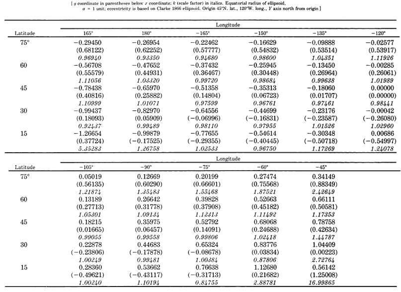
TABLE 34.— GS50 projection for 50 States: Rectangular coordinates for Clarke 1866 ellipsoid
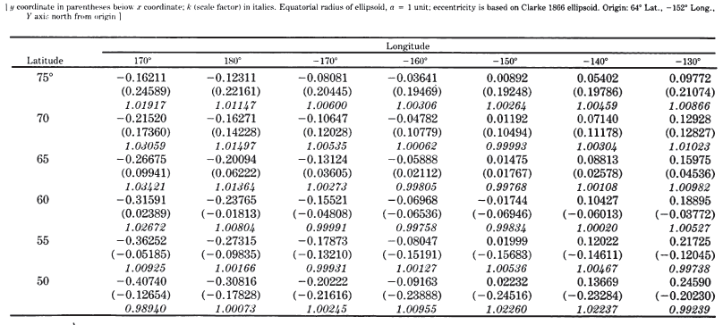
TABLE 35.— Modified-Stereographic Conformal projection for Alaska: Rectangular coordinates for Clarke 1866 ellipsoid