28. SATELLITE-TRACKING PROJECTIONS #
SUMMARY #
- All groundtracks for satellites orbiting the Earth with the same orbital parameters are shown as straight lines on the map. Cylindrical or conical form available.
- Neither conformal nor equal-area. All meridians are equally spaced straight lines, parallel on cylindrical form and
- converging to a common point on conical form. All parallels are straight and parallel on cylindrical form and are concentric circular arcs on conical form. Parallels are unequally spaced.
- Conformality occurs along two chosen parallels. Scale is correct along one of these parallels on the conical form and along both on the cylindrical form.
- Developed 1977 by Snyder.
HISTORY, FEATURES, AND USAGE #
The Landsat mapping system which inspired the development of the Space Oblique Mercator (SOM) projection also inspired the development of a simpler type of projection with a different purpose. While the SOM is used for low-distortion mapping of the strips scanned by the satellite, the Satellite-Tracking projections are designed solely to show the groundtracks for these or other satellites as straight lines, thus facilitating their plotting on a map. As a result, the other features of such maps are minimal, although they may be designed to reduce overall distortion in particular regions.
The writer developed the formulas in 1977 after essentially completing the mathematical development of the formulas for the SOM. The formulas for the Satellite-Tracking projections, with derivations, were published later (Snyder, 1981a). Arnold (1984) further analyzed the distortion. These formulas are confined to circular orbits and the spherical Earth. Because of the small-scale maps resulting, the ellipsoidal forms are hardly justified.
Charts of groundtracks have to date continued to employ the Lambert Conformal Conic projection, on which the groundtracks are slightly curved. The writer is not aware of any use of the new projection, except that a Chinese map of about 1982 claims this feature.
The projections were developed in two basic forms, the cylindrical and the conic, with variations of features within the latter category. The cylindrical form (fig. 48) has straight parallel equidistant meridians and straight parallels of latitude which are perpendicular to the meridians. The parallels of latitude are increasingly spaced away from the Equator, and for Landsat orbits the spacing changes more rapidly than it does on the Mercator projection. The Equator or two parallels of latitude equidistant from the Equator may be made standard, without shape or scale distortion, as on several other cylindrical projections. FIGURE 48.— Cylindrical Satellite-Tracking projection (standard parallels 30° N. and S.). Landsat 1, 2, 3 orbits. Groundtracks (paths 15, 30, 45, etc.) are shown as straight diagonal lines. They continue broken at tracking limits (not shown).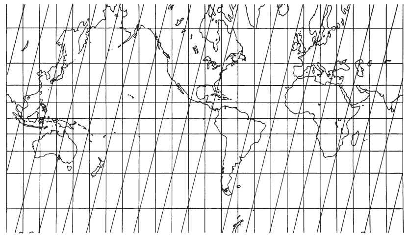
The groundtracks for the various orbits are plotted on the cylindrical form as diagonal equidistant straight lines. The descending orbital groundtracks (north to south) are parallel to each other, and the ascending groundtracks (south to north) are parallel to each other but with a direction in mirror image to that of the descending lines. The ascending and descending groundtracks meet at the northern and southern tracking limits, lats. 80.9° N. and S. for Landsat 1, 2, and 3. The map projection does not extend closer to the poles, although the mapmaker can arbitrarily extend the map using any convenient projection. The extension does not affect the purpose of the projection.
The groundtracks are not shown at constant scale, just as the straight great-circle paths on the Gnomonic and straight rhumb lines on the Mercator projection are not at constant scale. The complete tracks appear to be a sequence of zig-zag lines, although for Landsat normally only the descending (daylight) groundtracks should be shown to reduce confusion, since interest is normally confined to them.
While the cylindrical form of the Satellite-Tracking projections is of more interest if much of the world is to be shown, the conic form applies to most continents and countries, just as do the usual cylindrical and conic projections. On each conic Satellite-Tracking projection, the meridians are equally spaced straight lines converging at a common point, and the parallels are unequally spaced circular arcs centered on the same point. There are three types of distortion patterns available with the conic form:
- For the normal map (fig. 49) of a continent or country, there can be conformality or no shape distortion along two chosen parallels, but correct scale at only one of them. The groundtracks break at the closest tracking limit, but the map cannot be extended to the other tracking limit in many cases, since it extends infinitely before reaching that latitude.
- If one of the parallels with conformality is made a tracking limit, the groundtracks do not break at this tracking limit, since there can be no distortion there (fig. 50).
- If both parallels with conformality are made the same, the projection has just one standard parallel. If this parallel is made the tracking limit, the conic projection becomes the closest approximation to an azimuthal projection (fig. 51). For Landsat orbits, the cone constant of such a limiting projection is about 0.96, so the developed cone is about 4 percent less than a full circle, and the projection somewhat resembles a polar Gnomonic projection. With orbits of lower inclination, the approach to azimuthal becomes less.
For each of the conics, the straight groundtracks are equidistant, they have constant inclinations to each meridian being crossed at a given latitude on a given map, and they are not at constant scale. They are also all tangent to a circle slightly smaller than the latitude circle for the tracking limit in case 1 above, and tangent to the tracking limit itself in cases 2 and 3. As in the case of the cylindrical form, any extension of the map from the tracking limit to a pole is cosmetic and arbitrary, since the groundtracks do not pass through this region. FIGURE 49.— Conic Satellite-Tracking projection (conformality at lats. 45° and 70° N. ) . Landsat 1, 2, 3 orbits. Groundtracks (paths 15, 30, 45, etc.) are shown as diagonal straight lines. They continue broken (not shown) at tracking limit, the smallest incomplete circle. The complete circle is the circle of tangency.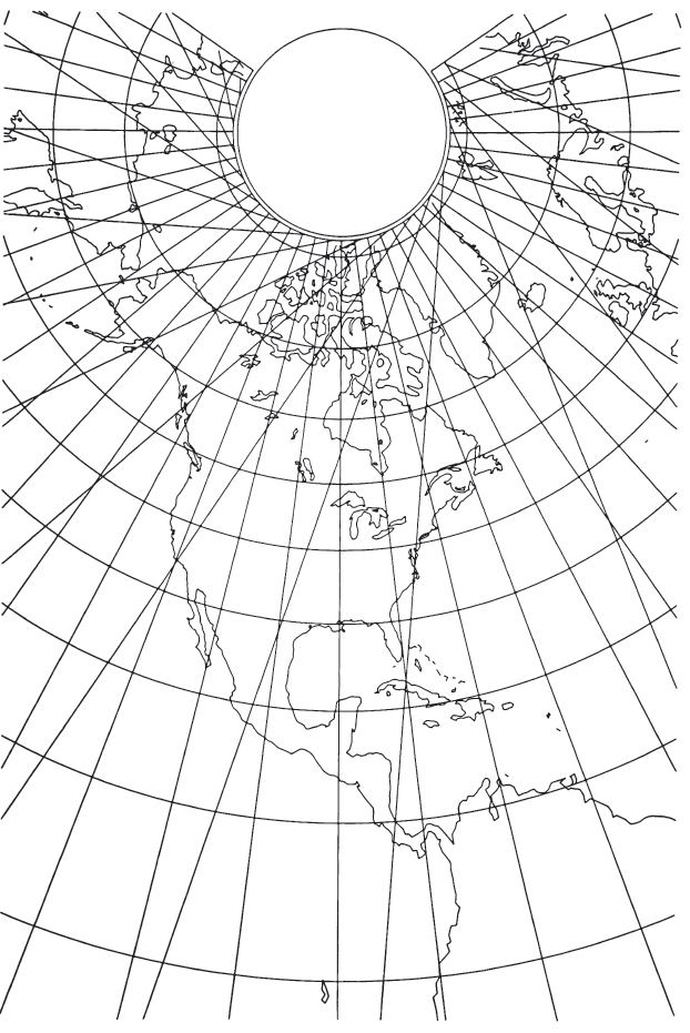
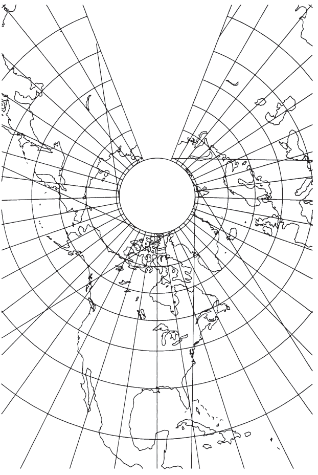
FIGURE 50.— Conic Satellite-Tracking projection (conformality at lats. 45° and 80.9° N.). Landsat 1,2,3 orbits. Diagonal groundtracks (paths 15,60,106,e tc.) are straight, unbroken even at the tracking limit, which is the same as the circle of tangency (inner circle).
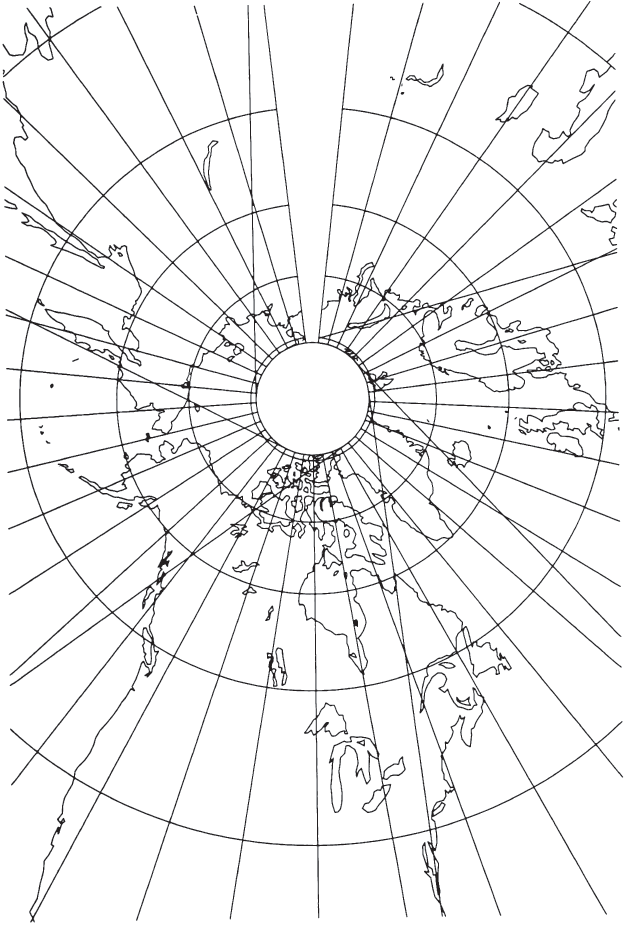
FIGURE 51.— Conic Satellite-Tracking projection (standard parallel 80.9° N.). Landsat 1, 2, 3 orbits. Groundtracks are as described on Fig. 50. The nearest approach to an azimuthal projection for these orbits. Inner circle is tracking limit and circle of tangency.
FORMULAS FOR THE SPHERE #
Forward formulas (see p. 360 for numerical examples): For the Cylindrical Satellite-Tracking projection, $R, i, P_2, P_1, \lambda_0, \phi_1, \phi,$ and $\lambda$ must be given, where
For the Conic Satellite-Tracking projection with two parallels having conformality, $R, i, P_2, P_1, \lambda_0, \phi_0, \phi_1, \phi_2, \phi,$ and $\lambda$ must be given, where the symbols are defined above, except that $\phi_2$ is the other parallel of conformality, but without true scale, and $\phi_0$ is the latitude crossing the central meridian at the desired origin of rectangular coordinates. For constants which apply to the entire map,
For plotting each point $(\phi, \lambda)$,
In addition, $\rho_s$ the radius of the circle to which groundtracks are tangent on the map, and scale factors h and k, defined above, are found as follows:
For the conic projection with one standard parallel, $\phi_1 = \phi_2$ but equation (28-10) is indeterminate. The following may be used in its place:
Inverse Formulas (see p. 362 for numerical examples):
For the cylindrical form, the same constants must be given as those listed for the forward formulas ($R, i, P_2, P_1, \lambda_0,$ and $\phi_1$), and $F’_1$ must be calculated from equation (28-1). For a given $(x, y)$, to find $(\phi, \lambda)$:
A generally faster solution of (28-20) and (28-21) involves the use of a Newton-Raphson iteration in place of those two equations, although equations are longer:
For any of the conic forms, the initial constants $R, i, P_2, P_1, \lambda_0, \phi_0,$ and $\phi_1$ alone or both $\phi_1$, and $\phi_2$ must be given. In addition, all constants in equations (28-9) through (28-12), (28-2a) through (28-4a), and (28-17) or (28-18) if necessary must be calculated. For a given $(x, y)$, to find $(\phi, \lambda)$,
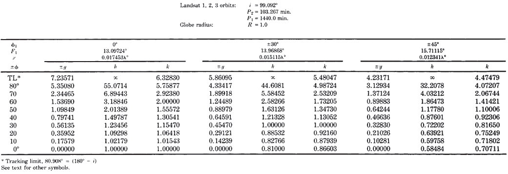
TABLE 38.— Cylindrical Satellite-Tracking projection: Rectangular coordinates
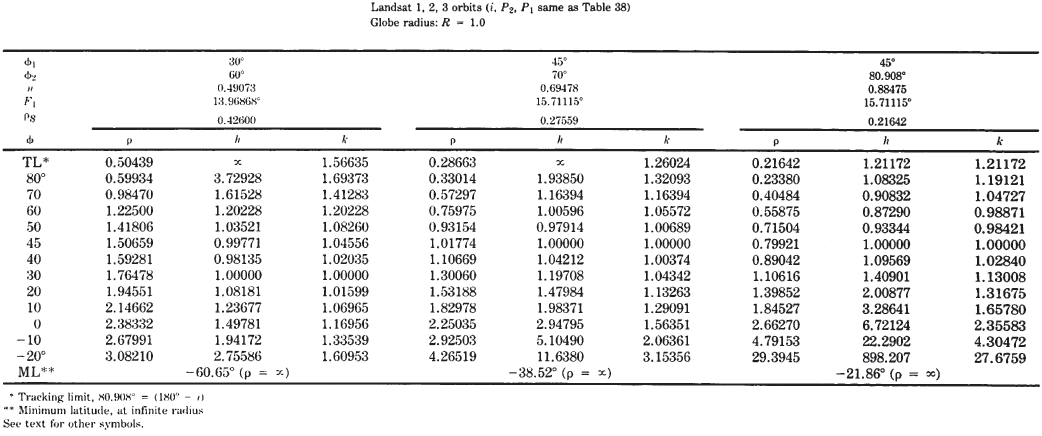
TABLE 39.— Conic Satellite-Tracking projections with Two conformal parallels: Polar coordinates
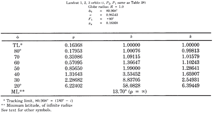
TABLE 40.— Near-Azimuthal Conic Satellite-Tracking projection: Polar coordinates