One of the most recent developments in map projections has been that involving a time factor, relating a mapping satellite revolving in an orbit about a rotating Earth. With the advent of automated continuous mapping in the near future, the static projections previously available are not sufficient to provide the accuracy merited by the imagery, without frequent readjustment of projection parameters and discontinuity at each adjustment. Projections appropriate for such satellite mapping are much more complicated mathematically, but, once derived, can be handled by computer.
Several such space map projections have been conceived, and all but one have been mathematically developed. The Space Oblique Mercator projection, suitable for mapping imagery from Landsat and other vertically scanning satellites, is described below, and is followed by a discussion of Satellite-Tracking projections. The Space Oblique Conformal Conic is a still more complex projection, currently only in conception, but for which mathematical development will be required if satellite side-looking imagery has been developed to an extent sufficient to encourage its use.
The launching of an Earth-sensing satellite by the National Aeronautics and Space Administration in 1972 led to a new era of mapping on a continuous basis from space. This satellite, first called ERTS-1 and renamed Landsat 1 in 1975, was followed by two others, all of which circled the Earth in a nearly circular orbit inclined about 99° to the Equator and scanning a swath about 185 km (officially 100 nautical miles) wide from an altitude of about 919 km. The fourth and fifth Landsat satellites involved circular orbits inclined about 98° and scanning from an altitude of about 705 km.
Continuous mapping of this band required a new map projection. Although conformal mapping was desired, the normal choice, the Oblique Mercator projection, is unsatisfactory for two reasons. First, the Earth is rotating at the same time the satellite is moving in an orbit which lies in a plane almost at a right angle to the plane of the Equator, with the double-motion effect producing a curved groundtrack, rather than one formed by the intersection of the Earth’s surface with a plane passing through the center of the Earth. Second, the only available Oblique Mercator projections for the ellipsoid are for limited coverage near the chosen central point.
What was needed was a map projection on which the groundtrack remained true-to-scale throughout its course. This course did not, in the case of Landsat 1,2, or 3, return to the same point for 251 revolutions. (For Landsat 4 and 5, the cycle is 233 revolutions.) It was also felt necessary that conformality be closely maintained within the range of the swath mapped by the satellite.
Alden P. Colvocoresses of the Geological Survey was the first to realize not only that such a projection was needed, but also that it was mathematically feasible. He defined it geometrically (Colvocoresses, 1974) and immediately began to appeal for the development of formulas. The following formulas resulted from the writer’s response to Colvocoresses’ appeal made at a geodetic conference at The Ohio State University in 1976. While the formulas were derived (1977-79) for Landsat, they are applicable to any satellite orbiting the Earth in a circular or elliptical orbit and at any inclination. Less complete formulas were also developed in 1977 by John L. Junkins, then of the University of Virginia. The following formulas are limited to nearly circular orbits. A complete derivation for orbits of any ellipticity is given by Snyder (1981b) and another summary by Snyder (1978b).
The Space Oblique Mercator (SOM) projection visually differs from the Oblique Mercator projection in that the central line (the groundtrack of the orbiting satellite) is slightly curved, rather than straight. For Landsat, this groundtrack appears as a nearly sinusoidal curve crossing the X axis at an angle of about 8°. The scanlines, perpendicular to the orbit in space, are slightly skewed with respect to the perpendicular to the groundtrack when plotted on the sphere or ellipsoid. Due to Earth rotation, the scanlines on the Earth (or map) intersect the groundtrack at about 86° near the Equator, but at 90° when the groundtrack makes its closest approach to either pole. With the curved groundtrack, the scanlines generally are skewed with respect to the X and Y axes, inclined about 4° to the Y axis at the Equator, and not at all at the polar approaches.
The orbit for Landsat 1, 2, and 3 intersected the plane of the Equator at an inclination of about 99°, measured as the angle between the direction of satellite revolution and the direction of Earth rotation. Thus the groundtrack reached limits of about lat. 81° N. and S. (180° minus 99°). The 185-km swath scanned by Landsat, about 0.83° on either side of the groundtrack, led to complete coverage of the Earth from about lat. 82° N. to 82° S. in the course of the 251 revolutions. With a nominal altitude of about 919 km, the time of one revolution was 103.267 minutes, and the orbit was designed to complete the 251 revolutions in exactly 18 days. Landsat 4 and 5, launched in 1982 and 1984, respectively, scanned the same width, but with an orbit of different radius and inclination, as stated above.
As on the normal Oblique Mercator, all meridians and parallels are curved lines, except for the meridian crossed by the groundtrack at each polar approach. While the straight meridians are 180° apart on the normal Oblique Mercator, they are about 167° apart on the SOM for Landsat 1, 2, and 3, since the Earth advanced
about 26° in longitude for each revolution of the satellite.
As developed, the SOM is not perfectly conformal for either the sphere or ellipsoid, although the error is negligible within the scanning range for either. Along the groundtrack, scale in the direction of the groundtrack is correct for sphere or ellipsoid, while conformality is correct for the sphere and within 0.0005 percent of correct for the ellipsoid. At l° away from the groundtrack, the Tissot Indicatrix (the ellipse of distortion) is flattened a maximum of 0.001 percent for the sphere and a maximum of 0.006 percent for the ellipsoid (this would be zero if conformal). The scale l° away from the groundtrack averages 0.015 percent greater than that at the groundtrack, a value which is fundamental to projection. As a result of the slight nonconformality, the scale l° away from the groundtrack on the ellipsoid then varies from 0.012 to 0.018 percent more than the scale along the groundtrack.
A prototype version of the SOM was used by NASA with a geometric analogy proposed by Colvocoresses (1974) while he was seeking the more rigorous mathematical development. This consisted basically of moving an obliquely tangent cylinder back and forth on the sphere so that a circle around it which would normally be tangent shifted to follow the groundtrack. This is suitable near the Equator but leads to errors of about 0. l percent near the poles, even for the sphere. In 1977, John B. Rowland of the USGS applied the Hotine Oblique Mercator (described previously) to Landsat 1, 2, and 3 orbits in five stationary zones, with smaller but significant errors (up to twice the scale variation of the SOM) resulting from the fact that the groundtrack cannot follow the straight central line of the HOM. In addition, there are discontinuities at the zone changes. This was done to fill the void resulting from the lack of SOM formulas.
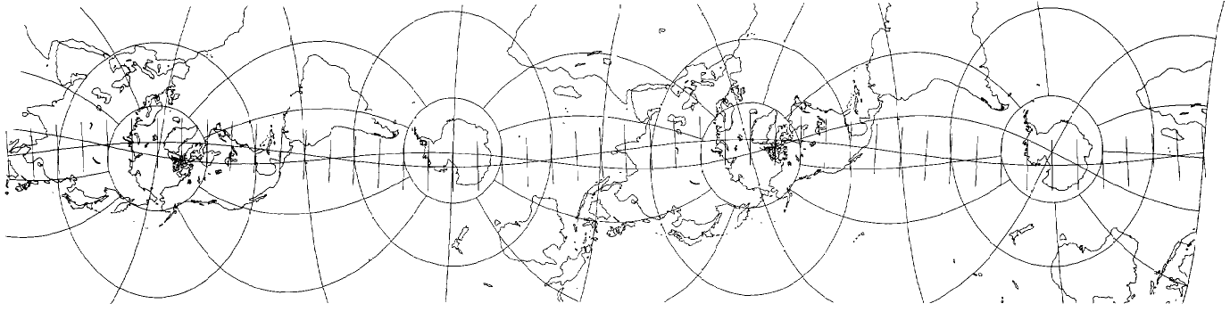
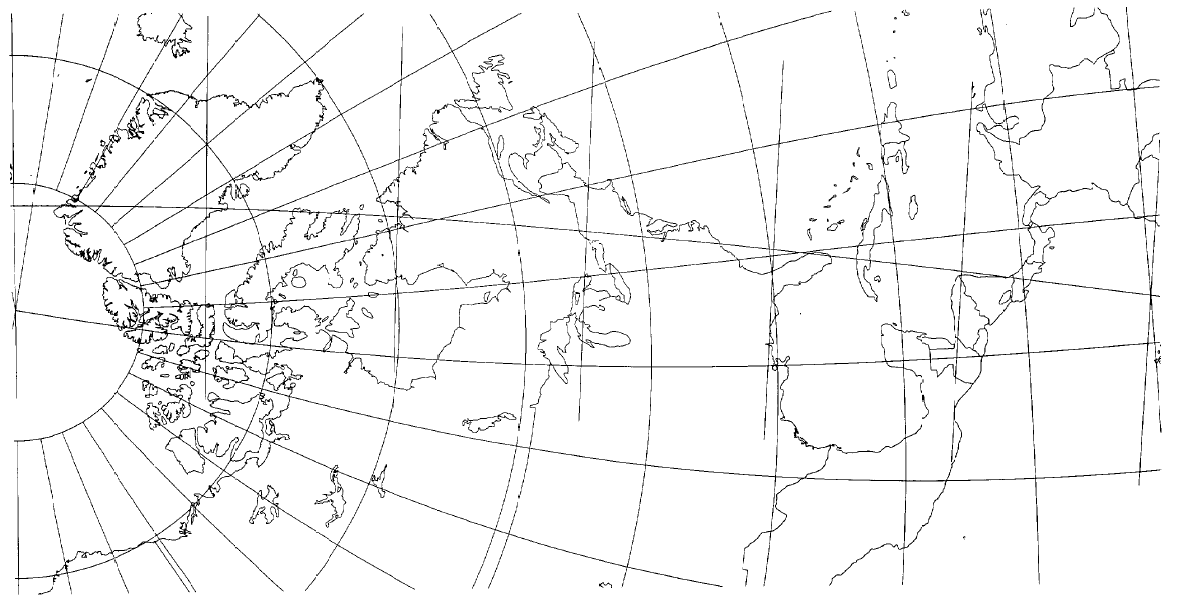
For Landsat 4 and 5, the final SOM equations replaced the HOM for mapping. Figures 46 and 47 show the SOM extended to two orbits with a 30° graticule and for one-fourth of an orbit with a 10° graticule, respectively. The progressive advance of meridians may be seen in figure 46. Both views are for Landsat 4 and 5 constants.
FIGURE 46.— Two orbits of the Space Oblique Mercator projection, shown for Landsat 5, paths 15 (left) and 31. Designed for a narrow band along groundtrack, which remains true to scale. Note the rotation of the Earth with successive orbits. Scan lines extended 15° from groundtrack are short lines nearly perpendicular to it.
FIGURE 47.— One quadrant of the Space Oblique Mercator projection for Landsat 5, path 15. An “enlargment” of part of figure 46 beginning at the North Pole.
Both iteration and numerical integration are involved in the formulas as presented for sphere or ellipsoid. The iteration is quite rapid (three to five iterations required for ten-place accuracy), and the numerical integration is greatly simplified by the use of rapidly converging Fourier series. The coefficients for the Fourier series may be calculated once for a given satellite orbit. [Some formulas below are slightly simplified from those first published (Snyder, 1978b).]
For the forward equations, for the sphere and circular orbit, to find $(x, y)$ for a given $(\phi,\lambda)$, it is necessary to be given $R, i, P_2, P_1, \lambda_0, \phi,$ and $\lambda$, where
$R=$
radius of the globe at the scale of the map.
$i=$
angle of inclination between the plane of the Earth’s Equator and the plane of the satellite orbit, measured counterclockwise from the Equator to the orbital plane at the ascending node (99.092° for Landsat l, 2, 3; 98.20° for Landsat 4, 5).
$P_2=$
time required for revolution of the satellite (103.267 min for Landsat 1, 2, 3; 98.884 min. for Landsat 4, 5).
$P_1=$
length of Earth’s rotation with respect to the precessed ascending node. For Landsat, the satellite orbit is Sun-synchronous; that is, it is always the same with respect to the Sun, equating $P_1$ to the solar day (1,440 min). The ascending node is the point on the satellite orbit at which the satellite crosses the Earth’s equatorial plane in a northerly direction.
$\lambda_0 = $
geodetic longitude of the ascending node at time $t = 0$.
$(\phi,\lambda)=$
geodetic latitude and longitude of point to be plotted on map.
$ t= $
time elapsed since the satellite crossed the ascending node for the orbit considered to be the initial one. This may be the current orbit or any earlier one, as long as the proper $\lambda_0$ is used.
First, various constants applying to the entire map for all the satellite’s orbits should be calculated a single time (see p. 347 for numerical examples):
$$ B = (2/\pi)\int_0^{\pi/2}[(H-S^2)/(1+S^2)^{1/2}]d\lambda' \tag{ 27-1 } $$
For calculating $A_n, B,$ and $C_n$ numerical integration using Simpson’s rule is recommended, with 9° intervals in $\lambda’$ (sufficient for ten-place accuracy). The terms shown are sufficient for seven-place accuracy, ample for the sphere. For H and S in equations (27-1) through (27-3):
$$ H = 1 - (P_2/P_1)\cos i \tag{ 27-4 } $$
$$ S = (P_2/P_1)\sin i \cos\lambda' \tag{ 27-5 } $$
To find $x$ and $y$, with the X axis passing through each ascending and descending node (wherever the groundtrack crosses the Equator), $x$ increasing in the direction of satellite motion, and the Y axis passing through the ascending node for time $t = 0$:
$$ \begin{align}
p \quad=\;&\text{path number of Landsat orbit for which the ascending node occurs at} \cr
&\text{time $t=0$. This ascending node is prior to the start of the path, so that} \cr
&\text{the path extends from 1/4 orbit past this node to 5/4 orbit past it.} \cr
\lambda' \quad=\;&\text{"transformed longitude," the angular distance along the groundtrack,} \cr
&\text{measured from the initial ascending node ($t = 0$), and directly proportional} \cr
&\text{to $t$ for a circular orbit, or $\lambda'=360^\circ t/P_2$.} \cr
\lambda_t\quad=\;&\text{a "satellite-apparent" longitude, the longitude relative to $\lambda_0$, seen by the} \cr
&\text{satellite if the Earth were stationary.} \cr
\phi'\quad=\;&\text{"transformed latitude," the angular distance from the groundtrack,}\cr
&\text{positive to the left of the satellite as it proceeds along the orbit.}
\end{align} $$
Finding $\lambda’$ from equations
(27-8) and
(27-9) involves iteration performed in the following manner: After selecting $\phi$ and $\lambda$, the $\lambda’$’ of the nearest polar approach, $\lambda_p’$, is used as the first trial $\lambda’$ on the right side of
(27-9); $\lambda_t$ is calculated and substituted into
(27-8) to find a new $\lambda’$’. A quadrant adjustment (see below) is applied to $\lambda’$, since the computer normally calculates arctan as an angle between -90° and 90°, and this $\lambda’$ is used as the next trial $\lambda’$ in
(27-9), etc., until $\lambda’$ changes by less than a chosen convergence factor. The value of $\lambda_p’$ may be determined as follows, for any number of revolutions:
where $N$ is the number of orbits completed at the last ascending node before the satellite passes the nearest pole, and the $\pm$ takes minus in the Northern Hemisphere and plus in the Southern (either for the Equator). Thus, if only the first path number past the ascending node is involved, $\lambda_p’$ is 90° for the first quadrant (North Pole to Equator), 270° for the second and third quadrants (Equator to South Pole to Equator), and 450° for the fourth quadrant (Equator to North Pole). For quadrant adjustment to $\lambda’$ calculated from
(27-8), the Fortran ATAN2 or its equivalent should not be used. Instead, $\lambda’$ should be increased by $\lambda_p’$ minus the following factor: 90° times $\sin $\lambda_p’$ $times $\pm,1$ (taking the sign of $cos \lambda_{tp}$, where $\lambda_{tp} = \lambda -\lambda_0 + (P2/P1)\lambda_p’$). If $\cos \lambda_{tp}$ is zero, the final $\lambda’$ is $\lambda_p’$. Thus, the adder to the arctan is 0° for the quadrant between the ascending node and the start of the path, and 180°, 180°, 360°, and 360°, respectively, for the four quadrants of the first path.
The closed forms of equations
(27-6) and
(27-7) are as follows:
Since these involve numerical integration for each point, the series forms, limiting numerical integration to once per satellite, are distinctly preferable. These are Fourier series, and equations
(27-2) and
(27-3) normally require integration from 0 to $2\pi$, without the multiplier 4, but the symmetry of the circular orbit permits the simplification as shown for the nonzero coefficients.
For inverse formulas for the sphere, given $R, i, P_2, P_1, \lambda_0, x,$ and $y$, with $\phi$ and $\lambda$ required: Constants $B, A_n, C_n$, and $\lambda_0$, must be calculated from
(27-1) through
(27-3) and
(27-11) just as they were for the forward equations. Then,
$$ \phi = \arcsin(\cos i \sin \phi' + \sin i \cos\phi'\sin\lambda') \tag{ 27-14 } $$
where the ATAN2 function of Fortran is useful for (27-13), except that it may be necessary to add or subtract 360° to place A between long. 180° E.(+) and 180° W.(-), and
Equation (27-15) is iterated by trying almost any $\lambda’$ (preferably $x/(BR)$) in the right side, solving for $\lambda’$ on the left and using the new $\lambda’$ for the next trial, etc., until there is no significant change between successive trial values. Equation (27-16) uses the final $\lambda’$ calculated from (27-15).
The closed form of equation (27-15) given below involves repeated numerical integration as well as iteration, making its use almost prohibitive:
The original published forms of these equations include several other Fourier coefficient calculations which slightly save computer time when continuous mapping is involved. The resulting equations are more complicated, so they are omitted here for simplicity. The above equations are as accurate and only slightly less
efficient.
The values of coefficients for Landsat 1,2, and 3 ($P_2/P_1= 18/251; i=99.092^\circ$) are listed here as examples:
It is also of interest to determine values of $\phi, \lambda$, or $\lambda’$ along the groundtrack, given any one of the three (as well as $P_2, P_1, i$, and $\lambda_0$). Given $\phi$,
If $\phi$ is given for a descending part of the orbit (daylight on Landsat), subtract $\lambda’$ from the $\lambda’$ of the nearest descending node (180°, 540°, …). If the orbit is ascending, add $\lambda’$ to the $\lambda’$ of the nearest ascending node (0°, 360°, …). For a given path, only 180° and 360°, respectively, are involved.
Given $\lambda’$, equations
(27-18) and
(27-20) may be used for $\lambda$ and $\phi$, respectively. Equations
(27-6) and
(27-7), with $\phi’ = 0$, convert these values to $x$ and $y$. Equations
(27-19) and
(27-9) require joint iteration, using the same procedure as that for the pair of equations
(27-8) and
(27-9) given earlier. The $\lambda$ calculated from equation
(27-18) should have the same quadrant adjustment as that described for
(27-13).
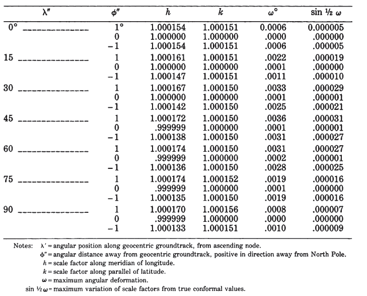
The formulas for scale factors $h$ and $k$ and maximum angular deformation $\omega$ are so lengthy that they are not given here. They are available in Snyder (1981b). Table 36 lists these values as calculated for the spherical SOM using Landsat constants. Although calculated for Landsat 1, 2, and 3, they are almost identical for 4 and 5.
TABLE 36.— Scale factors for the spherical Space Oblique Mercator projection using Landsat 1, 2, and 3 constants
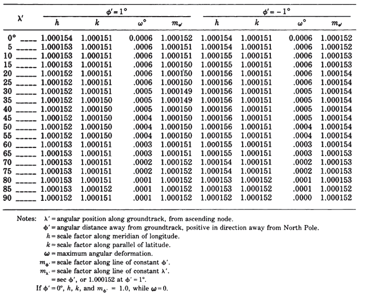
Since the SOM is intended to be used only for the mapping of relatively narrow strips, it is highly recommended that the ellipsoidal form be used to take advantage of the high accuracy of scale available, especially as the imagery is further developed and used for more precise measurement. In addition to the normal modifications to the above spherical formulas for ellipsoidal equivalents, an additional element is introduced by the fact that Landsat is designed to scan vertically, rather than in a geocentric direction. Therefore, “pseudotransformed” latitude $\phi^{\prime\prime}$ and longitude $\lambda^{\prime\prime}$ have been introduced. They relate to a geocentric groundtrack for an orbit in a plane through the center of the Earth. The regular transformed coordinates $\phi’$ and $\lambda’$ are related to the actual vertical groundtrack. The two groundtracks are only a maximum of 0.008° apart, although a lengthwise displacement of 0.028° for a given position may occur.
If the eccentricity of the ellipsoid is made zero, the formulas reduce to the spherical formulas above. These formulas vary slightly, but not significantly, from those published in Snyder (1978b, 1981b). In practice, the coordinates for each picture element (pixel) should not be calculated because of computer time required. Linear interpolation between occasional calculated points can be developed with adequate accuracy.
For the forward formulas, given $a, e, i, P_2, P_1, \lambda_0, R_0, \phi$, and $\lambda$, find $x$ and $y$. As with the spherical formulas, the X axis passes through each ascending and descending node, x increasing in the direction of satellite motion, and the Y axis intersects perpendicularly at the ascending node for the time $t = 0$. Defining terms,
$$ \begin{align}
a, e\, &=& &\text{semimajor axis and eccentricity of ellipsoid, respectively (as for other} \cr
& & &\text{ellipsoidal projections)} \cr
R_0\,&=& &\text {radius of the circular orbit of the satellite.}
\end{align} $$
$i, P_2, P_1, \lambda_0, \phi, \lambda$ are as defined for the spherical SOM formulas. For constants applying to the entire map (see p. 354 for numerical examples):
where $\phi’’$ and $\lambda’’$ are determined in these last two equations for the groundtrack as functions of $\lambda’$, from equations
(27-43),
(27-34),
(27-35), and
(27-36).
To calculate $A_n, B$, and $C_n$, the following functions, varying with $\lambda’’$, are used:
$$ S=(P_2/P_1)\sin i \cos\lambda''\{(1+T\sin^2{\lambda''})/[(1+W\sin^2{\lambda''})(1+Q\sin^2{\lambda''})]\}^{1/2} \tag{ 27-30 } $$
These constants may be determined from numerical integration, using Simpson’s rule with 9° intervals. For circular orbits, $A_n$ if $n$ is odd, $C_n$ if n is even, $j_n$ if $n$ is even, and $m_n$ if $n$ is odd are all zero. The above integration to $\pi/2$ is suitable, due to symmetry, only for non-zero coefficients. Integration to $2\pi$ would be necessary to show that other coefficients are zero.
Equations
(27-34) and
(27-35) are iterated together as were
(27-8) and
(27-9). Equation
(27-30) is used to find $S$ for the given $\lambda$ in equations
(27-32) and
(27-33). For improved computational efficiency using these and subsequent series, see p. 19.
The closed forms of equations
(27-32) and
(27-33) are given below, but the repeated numerical integration necessitates replacement by the series forms.
While the above equations are sufficient for plotting a graticule according to the SOM projection, it is also desirable to relate these points to the true vertical
groundtrack. To find $\phi’’$ and $\lambda’’$ in terms of $\phi’$ and $\lambda’$, the shift between these two sets of coordinates is so small it is equivalent to an adjustment, requiring only small Fourier coefficients, and very lengthy calculations if they are not used. The use of Fourier series is therefore highly recommended, although the one-time calculation of coefficients is more difficult than the foregoing calculation of $A_n, B,$ and $C_n$.
For a circular orbit, $\lambda’$ is $2\pi t/P_2$, where $t$ is the time from the initial ascending node.
The equations for functions of the satellite groundtrack, both forward and inverse, are given here, since some are used in calculating $j_n$, and $m_n$ as well. In any case $a, e, i, P_2, P_1, \lambda_0,$ and $R_0$ must be given. For $\lambda’$ and $\lambda$, if $\phi$ is given:
where $\phi_g$ is the geocentric latitude of the point geocentrically under the satellite, not the geocentric latitude corresponding to the vertical groundtrack latitude $\phi$.
These two equations are iterated as a group, but the first trial $\lambda’$ and the quadrant adjustments should follow the procedures listed for equation
(27-8).
Iteration is involved in (27-44), beginning with a trial $\phi$ of $\arcsin (\sin i \sin \lambda’)$.
If $\lambda’$ of a point along the groundtrack is given, $\phi$ is found from (27-44), and (27-43) provides $\lambda$. Only (27-44) requires iteration for these calculations.
Inverse formulas for the ellipsoidal form of the SOM projection, with circular orbit, follow: Given: $a, e, i, P_2, P_1, \lambda_0, R_0, x,$ and $y$, to find $\phi$ and $\lambda$, the general Fourier and other constants are first determined as described at the beginning of the forward equations. Then
No iteration is involved in equations (27-45) through (27-50), and the ATAN2 function of Fortran should be used with (27-46), but not (27-49), adding or subtracting
360° to or from $\lambda$ if necessary in (27-45) to place it between longs. 180° E. and W.
Iteration is required to find $\lambda’’$ from $x$ and $y$:
using equation
(27-30) and various constants. Iteration involves substitution of a trial $\lambda’’=x/a,B$ in the right side, finding a new $\lambda’’$ on the left side, etc.
For $\phi’’$, the $\lambda’’$ just calculated is used in the following equation:
Equations (27-53) and (27-54) are, of course, not the exact inverses of
(27-39) and
(27-40), although the correct coefficients may be derived by an analogous numerical integration in terms of $\lambda’’$, rather than $\lambda’$. The inverse values of $\phi’$ and $\lambda’$ from
(27-53) and
(27-54) are within 0.000003" and 0.000009°, respectively, of the true inverses of
(27-39) and
(27-40) for the Landsat orbits.
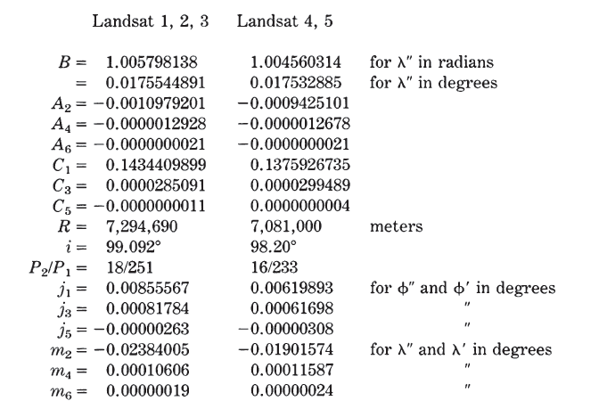
The following values of Fourier coefficients for the ellipsoidal SOM are listed for Landsat orbits, using the Clarke 1866 ellipsoid ($a=6,378,206.4$ m and $e^2=0.00676866$) and a circular orbit:
Additional Fourier constants have been developed in the published literature for other functions of circular orbits. They add to the complication of the equations, but not to the accuracy, and only slightly to continuous mapping efficiency. A further simplification from published formulas is the elimination of a function F, which nearly cancels out in the range involved in imaging.
As in the spherical form of SOM, the formulas for scale factors $h$ and $k$ and maximum angular deformation $\omega$ are too lengthy to include here, although they are given by Snyder (1981b). Table 37 presents these values for Landsat constants for the scanning range required. Values for Landsat 4 and 5 are nearly identical with those shown for 1, 2, and 3.
TABLE 37.— Scale factors for the ellipsoidal Space Oblique Mercator projection using Landsat 1, 2, and 3 constants
FORMULAS FOR THE ELLIPSOID AND NONCIRCULAR ORBIT
#
The following formulas accommodate a slight ellipticity in the satellite orbit. They provide a true-to-scale groundtrack for an orbit of any eccentricity, if the orbital motion follows Kepler’s laws for two-bodied systems, but the areas scanned by the satellite as shown on the map are distorted beyond the accuracy desired if the eccentricity of the orbit exceeds about 0.05, well above the maximum reported eccentricity of Landsat orbits (about 0.002). For greater eccentricities, more complex formulas (Snyder, 1981b) are recommended. If the orbital eccentricity is made zero, these formulas readily reduce to those for a circular orbit.
For the forward formulas, given $a, e, i, P_2, P_1, \lambda_0, a’, e’, \gamma, \phi,$ and $\lambda$, find $x$ and $y$. Again, the X axis passes through each ascending and descending node, x increasing in the direction of satellite motion, and the Y axis intersects perpendicularly at the ascending node for the time t = 0. Defining terms,
$$ \begin{align}
a', e'\;&=\;\text{semimajor axis and eccentricity of satellite orbit, respectively} \cr
\gamma &=\;\text{longitude of the perigee relative to the ascending node.}
\end{align} $$
$a$ and $e$ are as defined for the ellipsoidal/circular formulas, and $i, P_2, P_1, \lambda_0, \phi,$ and $\lambda$ are as defined for the spherical SOM formulas. For constants applying to the entire map (a numerical example is not given for the non-circular orbit):
$$ L' = (1-e'\cos{E'})^2/(1-e'^2)^{1/2} \tag{ 27-68 } $$
$$ E' = 2\arctan\{ \tan[(\lambda''-\gamma)/2][(1-e')/(1+e')]^{1/2}\} \tag{ 27-69 } $$
These constants may be determined from numerical integration, using Simpson’s rule with 9° intervals. Unlike the case for circular orbits, integration must occur through the 360° or $2\pi$ cycle, as indicated. Many more terms are needed than for circular orbits.
$$ E' = 2\arctan\{ \tan[(\lambda''-\gamma)/2][(1-e')/(1+e')]^{1/2}\} \tag{ 27-76 } $$
$$ \phi'' = \arcsin\{[(1-e^2)\cos i \sin \phi - \sin i \cos \phi\sin\lambda_t]/(1-e^2\sin^2\phi)^{1/2}\} \tag{27-36} $$
Function $E’$ is called the “eccentric anomaly” along the orbit, and $L$ is the “mean anomaly” or mean longitude of the satellite measured from perigee and directly proportional to time.
Equations
(27-34),
(27-74) through
(27-76), and
(27-36) are solved by special iteration as described for equations
(27-8) and
(27-9) in the spherical formulas, except that $\lambda’’$ replaces $\lambda’$, and each trial $\lambda’’$ is placed in
(27-76), from which $E’$ is calculated, then $L$, from
(27-75), $\lambda_t$ from
(27-74), and another trial $\lambda’’$ from
(27-34). This cycle is repeated until $\lambda’’$ changes by less than the selected convergence. The last value of $\lambda_t$ found is then used in
(27-36) to find $\phi’’$.
Equation
(27-67) is used to find $S$ for the given $\lambda’’$ in equations
(27-72) and
(27-73).
The closed forms of equations
(27-72) and
(27-73) are
(27-32a) and
(27-33a), respectively, in which the repeated numerical integration necessitates replacement by the series forms.
As in the case of the circular orbit, it is also desirable to relate these points to the true vertical groundtrack. To find $\phi’’$ and $\lambda’’$ in terms of $\phi’$ and $\lambda’$, the following series are employed:
$$ E' = e'\sin E' + L_0+2\pi t/P_2 \tag{ 27-80 } $$
$$ L_0 = E'_0-e'\sin E'_0 \tag{ 27-81 } $$
$$ E'_0 = -2\arctan\{ \} \tag{ 27-82 } $$
Equation (27-80) requires iteration, converging rapidly by substituting an initial trial $E’ = L_0 + 2\pi t/P_2$, in the right side, finding a new E’ on the left, substituting it on the right, etc., until sufficient convergence occurs.
The equations for functions of the satellite groundtrack, both forward and inverse, are given here, since some are used in calculating $j_m$ and $m_n$ as well. In
any case $a, e, i, P_2 P_1, \lambda_0 a’, e’,$ and $\gamma$ must be given. For $\lambda’$ and $\lambda$, if $\phi$ is given:
$$ E' = 2\arctan\{ \tan[(\lambda'-\gamma)/2][(1-e')/(1+e')]^{1/2}\} \tag{ 27-69a } $$
where $\phi_g$ is the geocentric latitude of the point geocentrically under the satellite, not the geocentric latitude corresponding to the vertical groundtrack latitude $\phi$, and $R_0$ is the radius vector to the satellite from the center of the Earth.
These equations are solved as a group by iteration, inserting a trial $\lambda’ = \arcsin(\sin\phi/\sin i)$ in (27-69a), solving (27-85), (27-84), and (27-83) for a new $\lambda’$, etc. Each trial $\lambda’$ must be adjusted for quadrant. If the satellite is traveling north, add 360° times the number of orbits completed at the nearest ascending node (0, 1, 2, etc.). If traveling south, subtract $\lambda’$ from 360° times the number of orbits completed at the nearest descending node (1/2, 3/2, 5/2, etc.). For $\lambda$,
and $L$ is found from (27-87) and (27-69a) above. The four equations are iterated as a group, as above, but the first trial $\lambda’$ and the quadrant adjustments should
follow the procedures listed for equation
(27-8).
where $R_0$ is determined from
(27-85) and
(27-69a), using the $\lambda’$ determined just above. Iteration is involved in (27-88), beginning with a trial $\phi$ of $\arcsin (\sin i \sin \lambda’)$.
If $\lambda’$ of a point along the groundtrack is given, \phi$ is found from
(27-88),
(27-85), and
(27-69a), while $\lambda$ is found from
(27-86),
(27-87), and
(27-69a). Only (27-88) requires iteration for these calculations.
Inverse formulas for the ellipsoidal form of the SOM projection, with an orbit of 0.05 eccentricity or less, follow: Given $a, e, i, P_2, P_1, \lambda_0, a’, e’, \gamma, x,$ and $y$, to find $\phi$ and $\lambda$, the general Fourier and other constants are first determined as described at the beginning of the forward equations for noncircular orbits. Then
No iteration is involved in equations (27-45) through (27-50), and the ATAN2 function of Fortran should be used with (27-46), but not (27-49), adding or subtracting
360° to or from $\lambda$ if necessary in (27-45) to place it between longs. 180° E. and W.
Iteration is required to find $\lambda’’$ from $x$ and $y$:
using equations
(27-67),
(27-92),
(27-93), and various constants. Iteration involves substitution of a trial $\lambda’’ = x’/B_1$ in the right side, finding a new $\lambda’’$ on the left side, etc.
For $\phi’’$, the $\lambda’’$ just calculated is used in the following equation:
For $\phi’$ and $\lambda’$ in terms of $\phi’’$ and $\lambda’’$, the same Fourier series developed for equations
(27-77) and
(27-78) may be used with reversal of signs, since the correction is so small. That is,
As with the circular orbit, equations (27-94) and (27-95) are not the exact inverses of
(27-77) and
(27-78), although the correct coefficients may be derived by an analogous numerical integration in terms of $\lambda’’$, rather than $\lambda’$.
All groundtracks for satellites orbiting the Earth with the same orbital parameters are shown as straight lines on the map. Cylindrical or conical form available.
Neither conformal nor equal-area. All meridians are equally spaced straight lines, parallel on cylindrical form and
converging to a common point on conical form. All parallels are straight and parallel on cylindrical form and are concentric circular arcs on conical form. Parallels are unequally spaced.
Conformality occurs along two chosen parallels. Scale is correct along one of these parallels on the conical form and along both on the cylindrical form.
The Landsat mapping system which inspired the development of the Space Oblique Mercator (SOM) projection also inspired the development of a simpler type of projection with a different purpose. While the SOM is used for low-distortion mapping of the strips scanned by the satellite, the Satellite-Tracking projections are designed solely to show the groundtracks for these or other satellites as straight lines, thus facilitating their plotting on a map. As a result, the other features of such maps are minimal, although they may be designed to reduce overall distortion in particular regions.
The writer developed the formulas in 1977 after essentially completing the mathematical development of the formulas for the SOM. The formulas for the Satellite-Tracking projections, with derivations, were published later (Snyder, 1981a). Arnold (1984) further analyzed the distortion. These formulas are confined to circular orbits and the spherical Earth. Because of the small-scale maps resulting, the ellipsoidal forms are hardly justified.
Charts of groundtracks have to date continued to employ the Lambert Conformal Conic projection, on which the groundtracks are slightly curved. The writer is not aware of any use of the new projection, except that a Chinese map of about 1982 claims this feature.
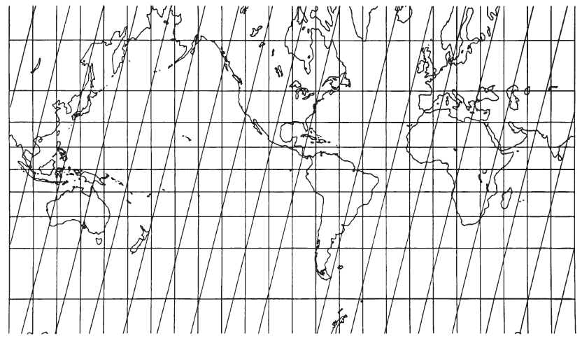
The projections were developed in two basic forms, the cylindrical and the conic, with variations of features within the latter category. The cylindrical form (fig. 48) has straight parallel equidistant meridians and straight parallels of latitude which are perpendicular to the meridians. The parallels of latitude are increasingly spaced away from the Equator, and for Landsat orbits the spacing changes more rapidly than it does on the Mercator projection. The Equator or two parallels of latitude equidistant from the Equator may be made standard, without shape or scale distortion, as on several other cylindrical projections.
FIGURE 48.— Cylindrical Satellite-Tracking projection (standard parallels 30° N. and S.). Landsat 1, 2, 3 orbits. Groundtracks (paths 15, 30, 45, etc.) are shown as straight diagonal lines. They continue broken at tracking limits (not shown).
The groundtracks for the various orbits are plotted on the cylindrical form as diagonal equidistant straight lines. The descending orbital groundtracks (north to south) are parallel to each other, and the ascending groundtracks (south to north) are parallel to each other but with a direction in mirror image to that of the descending lines. The ascending and descending groundtracks meet at the northern and southern tracking limits, lats. 80.9° N. and S. for Landsat 1, 2, and 3. The map projection does not extend closer to the poles, although the mapmaker can arbitrarily extend the map using any convenient projection. The extension does
not affect the purpose of the projection.
The groundtracks are not shown at constant scale, just as the straight great-circle paths on the Gnomonic and straight rhumb lines on the Mercator projection are not at constant scale. The complete tracks appear to be a sequence of zig-zag lines, although for Landsat normally only the descending (daylight) groundtracks should be shown to reduce confusion, since interest is normally confined to them.
While the cylindrical form of the Satellite-Tracking projections is of more interest if much of the world is to be shown, the conic form applies to most continents and countries, just as do the usual cylindrical and conic projections. On each conic Satellite-Tracking projection, the meridians are equally spaced straight lines converging at a common point, and the parallels are unequally spaced circular arcs centered on the same point. There are three types of distortion patterns available with the conic form:
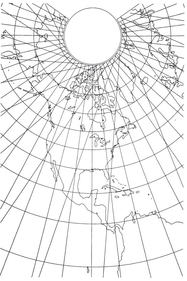
For the normal map (fig. 49) of a continent or country, there can be conformality or no shape distortion along two chosen parallels, but correct scale at only one of them. The groundtracks break at the closest tracking limit, but the map cannot be extended to the other tracking limit in many cases, since it extends infinitely before reaching that latitude.
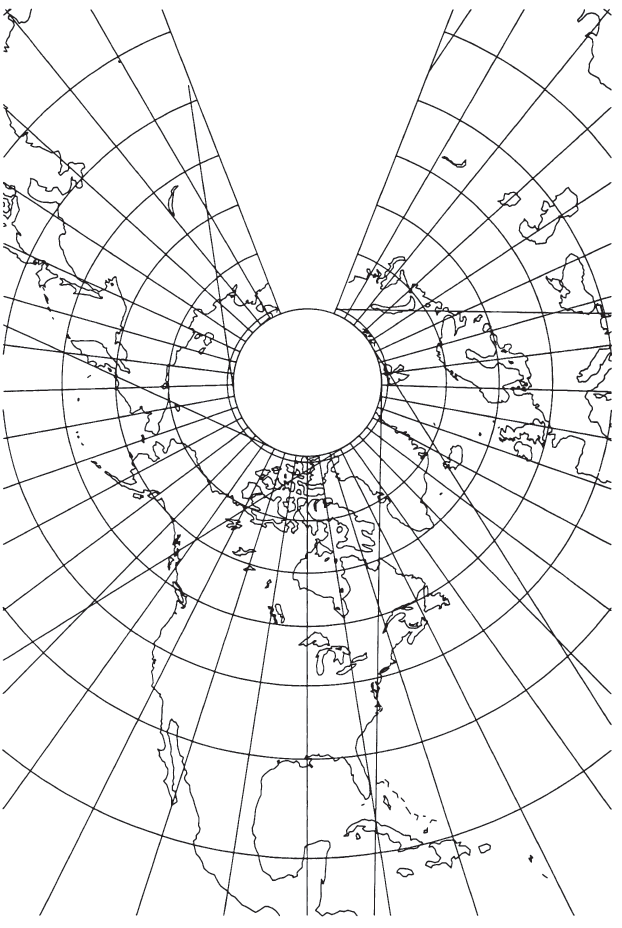
If one of the parallels with conformality is made a tracking limit, the groundtracks do not break at this tracking limit, since there can be no distortion there (fig. 50).
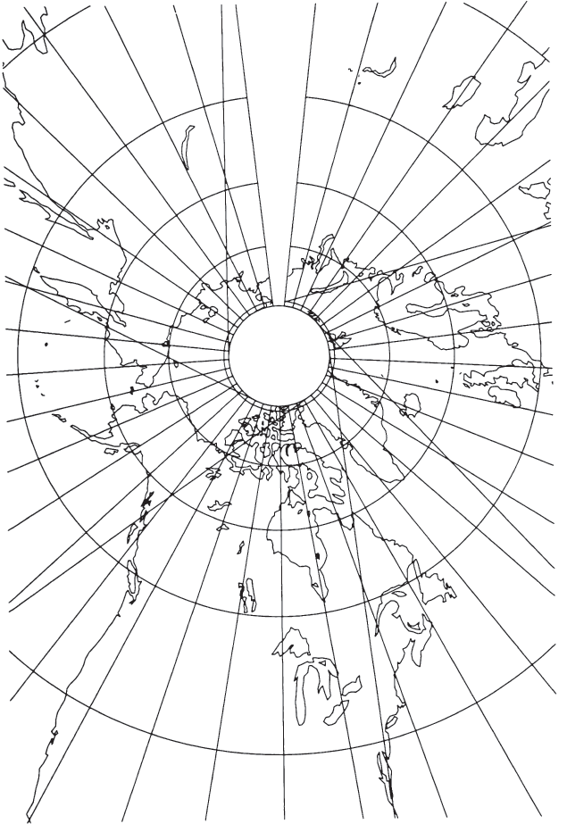
If both parallels with conformality are made the same, the projection has just one standard parallel. If this parallel is made the tracking limit, the conic projection becomes the closest approximation to an azimuthal projection (fig. 51). For Landsat orbits, the cone constant of such a limiting projection is about 0.96, so the developed cone is about 4 percent less than a full circle, and the projection somewhat resembles a polar Gnomonic projection. With orbits of lower inclination, the approach to azimuthal becomes less.
For each of the conics, the straight groundtracks are equidistant, they have constant inclinations to each meridian being crossed at a given latitude on a given map, and they are not at constant scale. They are also all tangent to a circle slightly smaller than the latitude circle for the tracking limit in case 1 above, and tangent to the tracking limit itself in cases 2 and 3. As in the case of the cylindrical form, any extension of the map from the tracking limit to a pole is cosmetic and arbitrary, since the groundtracks do not pass through this region.
FIGURE 49.— Conic Satellite-Tracking projection (conformality at lats. 45° and 70° N. ) . Landsat 1, 2, 3 orbits. Groundtracks (paths 15, 30, 45, etc.) are shown as diagonal straight lines. They continue broken (not shown) at tracking limit, the smallest incomplete circle. The complete circle is the circle of tangency.
FIGURE 50.— Conic Satellite-Tracking projection (conformality at lats. 45° and 80.9° N.). Landsat 1,2,3 orbits. Diagonal groundtracks (paths 15,60,106,e tc.) are straight, unbroken even at the tracking limit, which is the same as the circle of tangency (inner circle).
FIGURE 51.— Conic Satellite-Tracking projection (standard parallel 80.9° N.). Landsat 1, 2, 3 orbits. Groundtracks are as described on Fig. 50. The nearest approach to an azimuthal projection for these orbits. Inner circle is tracking limit and circle of tangency.
Forward formulas (see p. 360 for numerical examples): For the Cylindrical Satellite-Tracking projection, $R, i, P_2, P_1, \lambda_0, \phi_1, \phi,$ and $\lambda$ must be given, where
$$ \begin{align}
R\quad =&\;\text{radius of the globe at the scale of the map.} \cr
i\quad =&\;\text{angle of inclination between the plane of the Earth's Equator and the}\cr
&\quad\text{plane of the satellite orbit, measured counterclockwise from the Equator} \cr
&\quad\text{to the orbital plane at the ascending node (99.092° for Landsat l, 2, 3;} \cr
&\quad\text{98.20° for Landsat 4, 5).} \cr
P_2\quad=&\;\text{time required for revolution of the satellite (103.267 min for Landsat 1,} \cr
&\quad\text{2, 3; 98.884 min. for Landsat 4, 5).} \cr
P_1\quad=&\;\text{length of Earth's rotation with respect to the precessed ascending node.} \cr
&\quad\text{For Landsat, the satellite orbit is Sun-synchronous; that is, it is always}\cr
&\quad\text{the same with respect to the Sun, equating $P_1$ to the solar day (1,440} \cr
&\quad\text{min). The ascending node is the point on the satellite orbit at which the}\cr
&\quad\text{satellite crosses the Earth's equatorial plane in a northerly direction.}\cr
\lambda_0=&\;\text{central meridian.}\cr
\phi_1=&\;\text{standard parallel (N. and S.).}\cr
(\phi,\lambda)\,=&\;\text{geodetic latitude and longitude of point to be plotted on map.}
\end{align} $$
$$ L = \lambda_t - (P_2/P_1)\lambda' \tag{ 28-4 } $$
$$ x = R(\lambda-\lambda_0)\cos\phi_1 \tag{ 28-5 } $$
$$ y = R L\cos\phi_1/F'_1 \tag{ 28-6 } $$
$$ k = \cos\phi_1/\cos\phi \tag{ 28-7 } $$
$$ h = k F'/F'_1 \tag{ 28-8 } $$
Geometrically, $F’$ is the tangent of the angle on the globe between the groundtrack and the meridian at latitude $\phi$, and $F’_1$ is the tangent of this angle both on the globe and on the map at latitude $\phi_1$. Scale factors $h$ and $k$ apply along the meridian and parallel, respectively. If the latitude is closer to either pole than the corresponding tracking limit, equation (28-2) cannot be solved, and the point cannot be mapped using these formulas. The X axis lies along the Equator, x increasing easterly, and the Y axis lies along the central meridian, y increasing northerly. If $(\lambda-\lambda_0)$ lies outside the range $\pm180°$, 360° should be added or subtracted so it will fall inside the range.
For the Conic Satellite-Tracking projection with two parallels having conformality, $R, i, P_2, P_1, \lambda_0, \phi_0, \phi_1, \phi_2, \phi,$ and $\lambda$ must be given, where the symbols are defined above, except that $\phi_2$ is the other parallel of conformality, but without true scale, and $\phi_0$ is the latitude crossing the central meridian at the desired origin of rectangular coordinates. For constants which apply to the entire map,
in which subscript $n$ in equations (28-9) and (28-2a) through (28-4a) is made 0, 1, or 2 as required for (28-10) through (28-12), and subscript $n$ is omitted for calculating $F$ and $L$ for formulas below.
If $n$ is positive and $L$ is equal to or less than $(-s_0/n)$, or if $n$ is negative and $L$ is equal to or greater than $(-s_0/n)$, the point cannot or should not be plotted. The limiting latitude $\phi$ for $L = (-s_0/n)$ may be found using
(28-20) through
(28-22) below.
In addition, $\rho_s$ the radius of the circle to which groundtracks are tangent on the map, and scale factors h and k, defined above, are found as follows:
$$ \rho_s = R \cos\phi_1(\sin F_1)/n \tag{ 28-14 } $$
$$ k = \rho n /(R\cos\phi) \tag{ 28-15 } $$
$$ h = k\tan F/\tan(n L + s_0) \tag{ 28-16 } $$
Radius $\rho_s$, may be inserted into equations (14-1) and (14-2) in place of $\rho$ for rectangular coordinates. The Y axis lies along the central meridian $\lambda_0$, y increasing northerly, and the X axis intersects perpendicularly at $\phi_0$, x increasing easterly. Geometrically, $F_1$ is the inclination of the groundtrack to the meridian at latitude and $n$ is the cone constant.
For the conic projection with one standard parallel, $\phi_1 = \phi_2$ but equation
(28-10) is indeterminate. The following may be used in its place:
For the conic projection with one standard parallel which is equal to the upper tracking limit, equation (28-17) may be considerably simplified to the following:
$$ n=\sin i/[(P_2/P_1)\cos i -1]^2 \tag{ 28-18 } $$
Other equations for the conic form remain the same.
Inverse Formulas (see p. 362 for numerical examples):
For the cylindrical form, the same constants must be given as those listed for the forward formulas ($R, i, P_2, P_1, \lambda_0,$ and $\phi_1$), and $F’_1$ must be calculated from equation
(28-1). For a given $(x, y)$, to find $(\phi, \lambda)$:
Equations (28-20) and (28-21) must be iterated as a pair, using (-90°) as the first trial $\lambda’$ in equation (28-20), solving for $\lambda_t$, inserting it into (28-21), finding a new $\lambda’$ without using the equivalent of the Fortran ATAN2 function, and using it in (28-20), until $\lambda’$ changes by a negligible amount. This final $\lambda’$ is used in (28-22) to find $\phi$.
A generally faster solution of (28-20) and (28-21) involves the use of a Newton-Raphson iteration in place of those two equations, although equations are longer:
$$ A = \tan[L+(P_2/P_1)\lambda']/\cos i \tag{ 28-24 } $$
The first trial $\lambda’$ is again (-90°) in equation (28-24) and (28-25). The adjustment $\Delta\lambda’$ is added to each successive trial until reasonable convergence occurs.
For any of the conic forms, the initial constants $R, i, P_2, P_1, \lambda_0, \phi_0,$ and $\phi_1$ alone or both $\phi_1$, and $\phi_2$ must be given. In addition, all constants in equations
(28-9) through
(28-12),
(28-2a) through
(28-4a), and
(28-17) or
(28-18) if necessary must be calculated. For a given $(x, y)$, to find $(\phi, \lambda)$,
$$ \rho = \pm[x^2+(\rho_0-y)^2]^{1/2} \quad \text{,taking the sign of n} \tag{ 14-10 } $$
$$ L = [\arcsin(R\cos\phi_1\sin F_1/(\rho n))-s_0]/n \tag{ 28-26 } $$
From $L, \lambda’$ and then $\phi$ are found using equations
(28-20) through
(28-22), or
(28-24),
(28-25), and
(28-22), with iteration as described above. Then
$$ \lambda = \lambda_0 + \theta/n \tag{ 14-9 } $$
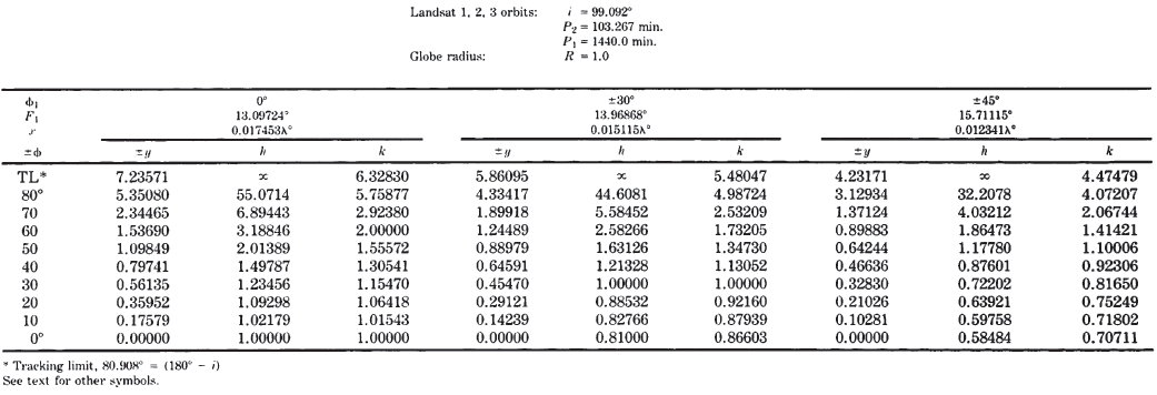
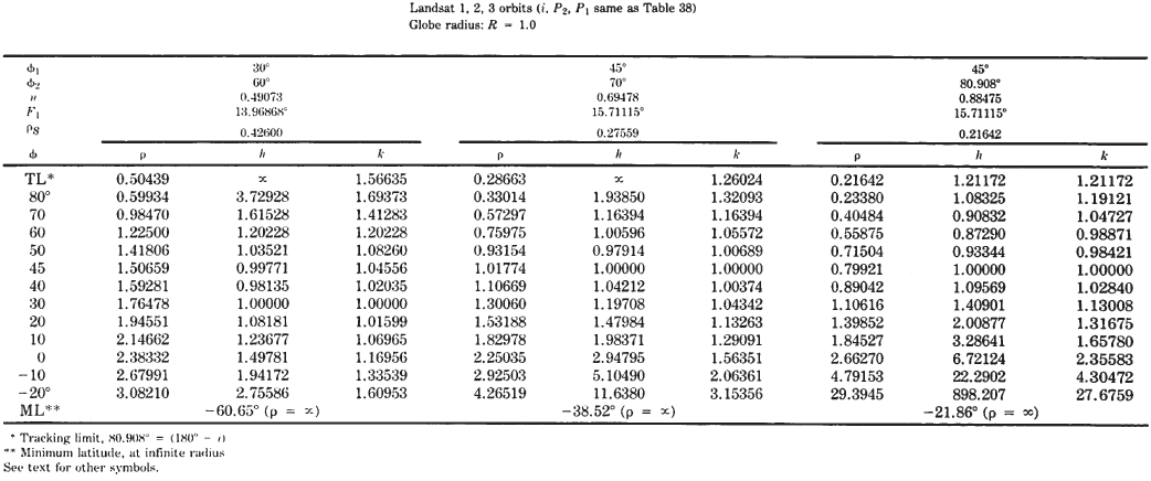
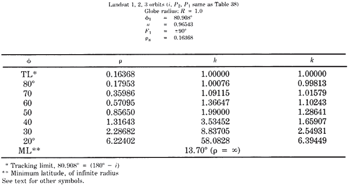
Sample coordinates for several of the Satellite-Tracking projections are shown in tables 38 through 40.
 Additional Fourier constants have been developed in the published literature for other functions of circular orbits. They add to the complication of the equations, but not to the accuracy, and only slightly to continuous mapping efficiency. A further simplification from published formulas is the elimination of a function F, which nearly cancels out in the range involved in imaging.