29. VAN DER GRINTEN PROJECTION #

SUMMARY #

Neither equal-area nor conformal. Not pseudocylindrical.
Shows entire globe enclosed in a circle.
Central meridian and Equator are straight lines.
All other meridians and parallels are arcs of circles.
A curved modification of the Mercator projection, with great distortion in the polar areas.
Equator is true to scale.
Used for world maps.
Used only in the spherical form.
Presented by van der Grinten in 1904.

HISTORY, FEATURES, AND USAGE #

In a 1904 issue of a German geographical journal, Alphons J. van der Grinten (1852-?) of Chicago presented four projections showing the entire Earth. Aside from having a straight Equator and central meridian, three of the projections consist of arcs of circles for meridians and parallels; the other projection has straight-line parallels. The projections are neither conformal nor equal-area (van der Grinten, 1904; 1905). They were patented in the United States by van der Grinten in 1904.

The best-known Van der Grinten projection, his first (fig. 52), shows the world in a circle and was invented in 1898. It is designed for use in the spherical form only. There are no special features to preserve in an ellipsoidal form. It has been used by the National Geographic Society for their standard world map since 1943, printed at various scales and with the central meridian either through America or along the Greenwich meridian; this use has prompted others to employ the projection. The U.S. Department of Agriculture adopted the projection as the base map for economic data in the 1940’s, and this led to frequent use in geography textbooks (Wong, 1965, p. 117). The USGS has used one of the National Geographic maps as a base for a four-sheet set of maps of World Subsea Mineral Resources, 1970, one at a scale of 1:60,000,000 and three at 1:39,283,200 (a scale used by the National Geographic), and for three smaller maps in the National Atlas (USGS, 1970, p. 150-151, 332-335). All the USGS maps have a central meridian of long. 85° W., passing through the United States.

FIGURE 52.— Van der Grinten projection. A projection resembling Mercator, but not conformal. Used by USGS for special world maps, modifying a base map prepared by the national Geographic Society. This illustration is prepared by computer.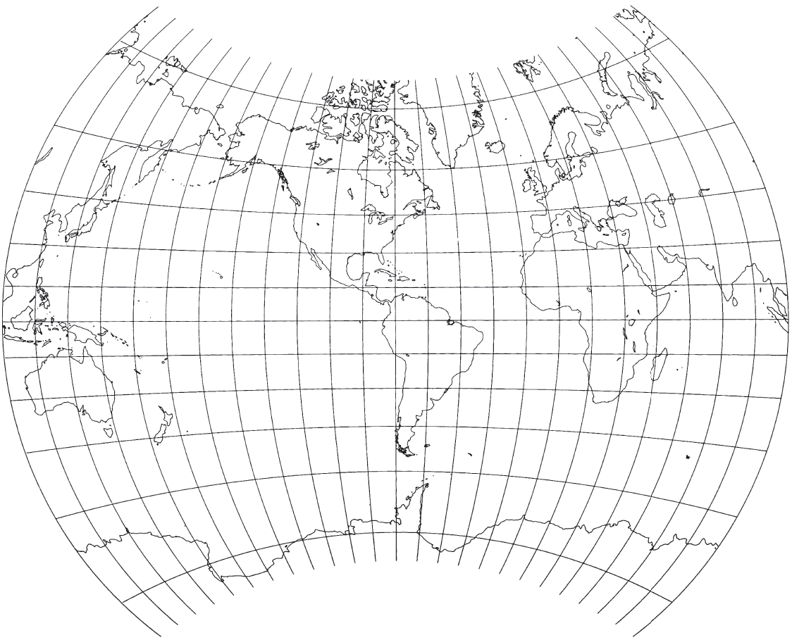 — **FIGURE 52**.— Van der Grinten projection. A projection resembling Mercator, but not conformal. Used by USGS for special world maps, modifying a base map prepared by the national Geographic Society. This illustration is prepared by computer.

Van der Grinten emphasized that this projection blends the Mercator appearance with the curves of the Mollweide, an equal-area projection described later. He included a simple graphical construction and limited formulas showing the mathematical coordinates along the central meridian, the Equator, and the outer (180th) meridian. The meridians are equally spaced along the Equator, but the spacing between the parallels increases with latitude, so that the 75th parallels are shown about halfway between the Equator and the respective poles. Because of the polar exaggerations, most published maps using the Van der Grinten projection do not extend farther into the polar regions than the northern shores of Greenland and the outer rim of Antarctica.

The National Geographic Society prepared the base map graphically. General mathematical formulas have been published in recent years and are only useful with computers, since they are fairly complex for such a simply drawn projection (O’Keefe and Greenberg, 1977; Snyder, 1979b).

GEOMETRIC CONSTRUCTION #

The meridians are circular arcs equally spaced on the Equator and joined at the poles. For parallels, referring to figure 53, semicircle CDB is drawn centered at A. Diagonal CD is drawn. Point E is marked so that the ratio of EA to AD is the same as the ratio of the latitude to 90°. Line FE is drawn parallel to CB, and FB and GB are connected. At H, the intersection of GB and AD, JHL is drawn parallel to CB. A circular arc, representing the parallel of latitude, is then drawn through JKL.

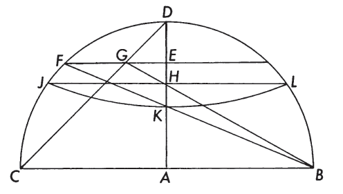
FORMULAS FOR THE SPHERE #

The general formulas published are in two forms. Both sets give identical results, but the 1979 formulas are somewhat shorter and are given here with some rearrangement and addition of new inverse equations. For the forward calculations, given $R, \lambda_0, \phi,$ and $\lambda$ (giving true scale along the Equator), to find $x$ and $y$ (see numerical examples):

$$ x = \pm\pi R\{A(G-P^2)+[A^2(G-P^2)^2-(P^2+A^2)(G^2-P^2)]^{1/2}\}/(P^2+A^2) \tag{ 29-1 } $$

taking the sign of $(\lambda-\lambda_0)$. Note that $(\lambda-\lambda_0)$ must fall between +180° and -180°; if necessary, 360° must be added or subtracted. The X axis lies along the Equator, x increasing easterly, while the Y axis coincides with the central meridian $\lambda_0$.

$$ y=\pm\pi R\{P Q - A[(A^2+1)(P^2+A^2)-Q^2]^{1/2}\}/(P^2+A^2) \tag{ 29-2 } $$

taking the sign of $\phi$,

where

$$ A = ½|\pi/(\lambda-\lambda_0)-(\lambda-\lambda_0)/\pi | \tag{ 29-3 } $$

$$ G = \cos\theta/(\sin\theta+\cos\theta-1) \tag{ 29-4 } $$

$$ P = G(2/\sin\theta-1) \tag{ 29-5 } $$

$$ \theta = \arcsin|2\phi/\pi| \tag{ 29-6 } $$

$$ Q = A^2+G \tag{ 29-6a } $$

But if $\phi = 0$ or $\pm90°$, or $\lambda = \lambda_0$, these equations are indeterminate. In that case, if $\phi=0$,

$$ x = R(\lambda-\lambda_0) \tag{ 29-7 } $$

and

$$ y = 0 $$

or if $\lambda=\lambda_0$ or $\phi = \pm90^\circ$

$$ x = 0 $$

and

$$ y=\pm\pi R\tan(\theta/2) \tag{ 29-8 } $$

taking the sign of $\phi$. It may be noted that absolute values (symbol $|\thinspace|$ ) are used in several cases. The origin is at the center $(\phi = 0, \lambda = \lambda_0)$.

For the inverse equations, given $R, \lambda_0, x,$ and $y,$ to find $\phi$ and $\lambda$: Because of the complications involved, the equations are given in the order of use. This is closely based upon a recent, noniterative algorithm by Rubincam (1981):

$$ X = x/(\pi R) \tag{ 29-9 } $$

$$ Y = y/(\pi R) \tag{ 29-10 } $$

$$ c_1 = -|Y|(1+X^2+Y^2) \tag{ 29-11 } $$

$$ c_2 = c_1 - 2Y^2+X^2 \tag{ 29-12 } $$

$$ c_3 = -2c_1+ 1 + 2Y^2+(X^2+Y^2)^2 \tag{ 29-13 } $$

$$ d = Y^2/c_3 + (2c_2^3/c_3^3-9c_1c_2/c_3^2)/27 \tag{ 29-14 } $$

$$ a_1 = (c_1-c_2^2/3c_3)/c_3 \tag{ 29-15 } $$

$$ m_1 = 2(-a_1/3)^{1/2} \tag{ 29-16 } $$

$$ \theta_1 = (1/3)\arccos(3d/a_1m_1) \tag{ 29-17 } $$

$$ \phi = \pm\pi[-m_1\cos(\theta_1+\pi/3)-c_2/3c_3] \tag{ 29-18 } $$

taking the sign of $y$.

$$ \lambda = \pi\{X^2+Y^2-1+[1+2(X^2-Y^2)+(X^2+Y^2)^2]^{1/2}\}/2X+\lambda_0 \tag{ 29-19 } $$

but if $X = 0$, equation (29- 19) is indeterminate. Then

$$ \lambda=\lambda_0 \tag{ 29-20 } $$

The formulas for scale factors are quite lengthy and are not included here. Rectangular coordinates are given in table 41 for a map of the world with unit radius of the outer circle. or $R = 1/\pi$. The longitude is measured from the central meridian. Only one quadrant of the map is given, but the map is symmetrical about both X and Y axes.

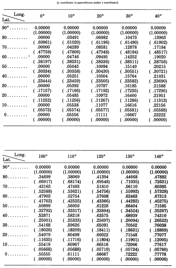
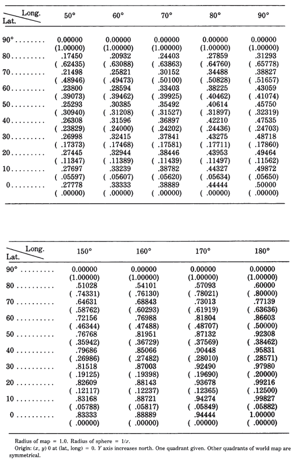
TABLE 41.— Van der Grinten projection: Rectangular coordinates — **TABLE 41**.— Van der Grinten projection: Rectangular coordinates