30. SINUSOIDAL PROJECTION #
SUMMARY #
- Pseudocylindrical projection.
- Equal-area.
- Central meridian is a straight line; all other meridians are shown as equally spaced sinusoidal curves.
- Parallels are equally spaced straight lines, parallel to each other. Poles are points.
- Scale is true along central meridian and all parallels.
- Used for world maps with single central meridian or in interrupted form with
- several central meridians.
- Used for maps of South America and Africa.
- Used since the mid-16th century.
HISTORY #
There is an almost endless number of possible projections with horizontal straight lines for parallels of latitude and curved lines for meridians. They are sometimes called pseudocylindrical because of their partial similarity to cylindrical projections. Scores of such projections have been presented, purporting various special advantages, although several are strikingly similar to other members of the group (Snyder, 1977). While there were rudimentary projections with straight parallels used as early as the 2nd century B.C. by Hipparchus, the first such projection still used for scientific mapping of the sphere is the Sinusoidal.
This projection (fig. 54) used for world maps as well as maps of continents and other regions, especially those bordering the Equator, has been given many names after various presumed originators, but it is most frequently called by the name used here. Among the first to show the Sinusoidal projection was Jean Cossin of Dieppe, who used it for a world map of 1570. In addition, it was used by Jodocus Hondius for maps of South America and Africa in some of his editions of Mercator’s atlases of 1606-1609. This is probably the basis for one of the names of the projection: The Mercator Equal-Area. Nicolas Sanson (1600-67) of France used it in about 1650 for maps of continents, while John Flamsteed (1646-1719) of England later used it for star maps. Thus, the name “Sanson-Flamsteed” has often been applied to the Sinusoidal projection, even though they were not the originators (Keuning, 1955, p. 24; Deetz and Adams, 1934, p. 161). FIGURE 54.— Interrupted Sinusoidal projection as used by USGS. The oldest pseudocylindrical projection, it shows areas correctly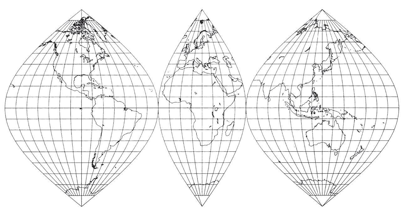
FEATURES AND USAGE #
The simplicity of construction, either graphically or mathematically, combined with the useful features obtained, make the Sinusoidal projection not only popular to use, but a popular object of study for interruptions, transformations, and combination with other projections.
On the normal Sinusoidal projection, the parallels of latitude are equally spaced straight parallel lines, and the central meridian is a straight line crossing the parallels perpendicularly. The Equator is marked off from the central meridian equidistantly for meridians at the same scale as the latitude markings on the central meridian, so the Equator for a complete world map is twice as long as the central meridian. The other parallels of latitude are also marked off for meridians in proportion to the true distances from the central meridian. The meridians connect these markings from pole to pole. Since the spacings on the parallels are proportional to the cosine of the latitude, and since parallels are equally spaced, the meridians form curves which may be called cosine, sine,or sinusoidal curves; hence, the name.
Areas are shown correctly. There is no distortion along the Equator and central meridian, but distortion becomes pronounced near the outer meridians, especially in the polar regions.
Because of this distortion, J. Paul Goode (1862-1932) of the University of Chicago developed an interrupted form of the Sinusoidal in 1916 with several meridians chosen as central meridians without distortion and a limited expanse east and west for each section. The central meridians may be different for Northern and Southern Hemispheres and may be selected to minimize distortion of continents or of oceans instead. Ultimately, Goode combined the portion of the interrupted Sinusoidal projection between about lats. 40° N. and S. with the portions of the Mollweide or Homolographic projection (described later) not in this zone, to produce the Homolosine projection used in Rand McNally’s Goode’s Atlas (Goode, 1925).
In 1927, the Sinusoidal was shown interrupted in three symmetrical segments in the Nordisk Världs Atlas, Stockholm, serving as the base for the Sinusoidal as shown in Deetz and Adams (1934, p. 161). It is this interrupted form which served in turn as the base for a three-sheet set by the USGS in 1978 at a scale of 1:20,000,000, entitled Map of Prospective Hydrocarbon Provinces of the World. With interruptions occurring at longs. 160° W., 20° W., and 60° E., and the three central meridians equidistant from these limits, the sheets show (1) North and South America; (2) Europe, West Asia, and Africa; and (3) East Asia, Australia, and the Pacific; respectively. The maps extend pole to pole, but no data are shown for Antarctica. An inset of the Arctic region at the same scale is drawn to the polar Lambert Azimuthal Equal-Area projection. A similar map is being prepared by the USGS showing sedimentary basins of the world.
The Sinusoidal projection is normally used in the spherical form, adequate for the usual small-scale usage, but the ellipsoidal form has been used for topographic mapping in Ecuador (C. J. Mugnier, pers. comm., 1985).
FORMULAS FOR THE SPHERE #
The formulas for the Sinusoidal projection are perhaps the simplest of those for any projection described in this bulletin, except for the Equidistant Cylindrical. For the forward case, given $R, \lambda_0, \phi,$ and $\lambda$ to find $x$ and $y$ (see numerical examples):
In equations (30-1) through (30-5), radians must be used, or $\phi$ and $\lambda$ in degrees must be multiplied by $\pi/180^\circ$.
For the inverse formulas, given $R, \lambda_0, x,$ and $y$, to find $\phi$ and $\lambda$:
FORMULAS FOR THE ELLIPSOID #
The ellipsoidal form may be made by spacing parallels along the central meridian(s) true to scale for the ellipsoid and meridians along each parallel also true to scale. The projection remains equal-area, while the parallels are not quite equally spaced, and the meridians are no longer perfect sinusoids. Specifically, given $a, e, \lambda_0, \phi,$ and $\lambda$, to find $x$ and $y$ (see numerical examples):
For the inverse formulas, given $a, e, \lambda_0, x,$ and $y$, to find $\phi$ and $\lambda$: