31. MOLLWEIDE PROJECTION #

SUMMARY #

Pseudocylindrical.
Equal-area.
Central meridian is a straight line; 90th meridians are circular arcs; all other meridians are equally spaced elliptical arcs.
Parallels are unequally spaced straight lines, parallel to each other. Poles are points.
Scale is true along latitudes 40°44’ N. and S.
Used for world maps with single central meridian or in interrupted form with several central meridians.
Inspiration for several other projections.
Presented by Mollweide in 1805.

HISTORY AND USAGE #

The second oldest pseudocylindrical projection which is still in use (after the Sinusoidal) was presented by Carl B. Mollweide (1774-1825) of Halle, Germany, in 1805 (Mollweide, 1805). It is an equal-area projection of the Earth within an ellipse. It has had a profound effect on world map projections in the 20th century, especially as an inspiration for other important projections. It lay dormant until J. Babinet reintroduced it in 1857 under the name “homalographic.” It has been called Babinet’s Equal-Surface or the Elliptical projection, but it is most often called the Mollweide, Homalographic, or Homolographic.

J. Paul Goode, after interrupting the Sinusoidal projection, made similar interruptions of the Mollweide in 1916 to minimize distortion of continents or oceans. Ultimately he combined them to produce the Homolosine projection.

Other projections directly inspired by the Mollweide have been the Van der Grinten, described earlier, and the Boggs Eumorphic, in which the y coordinates of the Sinusoidal and Mollweide are arithmetically averaged, and the x coordinates are derived to maintain equality of area (Boggs, 1929). J. Fairgrieve in 1928 (Steers, 1970, p. 172) was the first of several to use the oblique aspect, and John Bartholomew applied the name “Atlantis” to a transverse Mollweide centered on the Atlantic Ocean and used as the frontispiece in The Times Atlas of 1958. Allen K. Philbrick (1953) combined the Sinusoidal and Mollweide in a manner different from the Goode Homolosine, using both normal and oblique aspects. Less direct inspiration by the Mollweide has led to several other projections, especially pseudocylindrical, some of which have lines for poles.

Some other projections showing the world in an ellipse, especially the Hammer and the Briesemeister, originate from the Lambert Azimuthal Equal-Area projection, not the Mollweide. Another projection occasionally seen is identical with the Mollweide, except that the parallels are equally spaced, and therefore the projection is not equal-area. It was first used in a rudimentary form in the 16th century.

FEATURES #

Unlike the Sinusoidal projection, which has been satisfactorily used for continental maps, the Mollweide projection (fig. 55) is normally used as a world map, and occasionally for a very large region such as the Pacific Ocean. This is because only two points on the Mollweide are completely free of distortion unless the projection is interrupted. These are the points at latitudes 40°44'12" N. and S. on the central meridian(s).

FIGURE 55.— Mollweide projection. An equal-are projection of the world bounded by an ellipse and the basis for several other projections.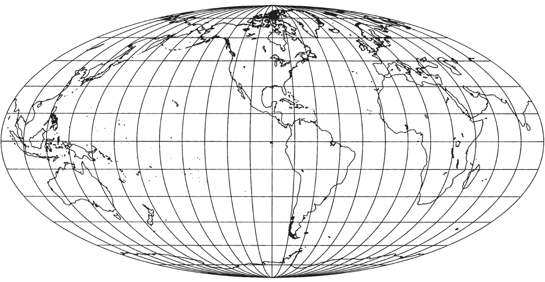 — **FIGURE 55**.— Mollweide projection. An equal-are projection of the world bounded by an ellipse and the basis for several other projections.

The world is shown in an ellipse with the Equator, its major axis, twice as long as the central meridian, its minor axis. The meridians 90° east and west of the central meridian form a complete circle. All other meridians are elliptical arcs which, with their opposite numbers on the other side of the central meridian, form complete ellipses which meet at the two poles. The central meridian is the major axis of meridian ellipses less than 90° from it, and a portion of the Equator is the minor axis. Meridians greater than 90° have the reverse arrangement for their axes. Meridians are equally spaced along the Equator and along all other parallels. The 90th meridians form a circle.

The parallels of latitude are straight parallel lines, but they are not equally spaced. Their spacing may be determined from the facts that the projection is equal-area and that the 90th meridians are circular. As a result, the regions along the Equator are stretched 23 percent in a north-south direction relative to east-west dimensions. This stretching decreases along the central meridian to zero at the 40°44’ latitudes, and becomes compression nearer the poles. The distortion near the outer meridians is considerable at high latitudes, but less than that on the Sinusoidal. The distortion along the Equator led Bromley (1965) to propose flattening the projection in a north-south direction and expanding east-west, to provide an Equator free of distortion, but the Equator thereby becomes 2.47 times as long as the central meridian.

Because the Mollweide projection is normally used at a small scale, there is little justification for an ellipsoidal form.

FORMULAS FOR THE SPHERE #

The forward formulas for the Mollweide require iteration, but they are otherwise relatively simple. Given $R, \lambda_0, \phi,$ and $\lambda$, to find $x$ and $y$ (see numerical examples):

$$ x = (8^{1/2}/\pi)R(\lambda-\lambda_0)\cos\theta \tag{ 31-1 } $$

$$ y = 2^{1/2}R\sin\theta \tag{ 31-2 } $$

where

$$ 2\theta+\sin2\theta = \pi\sin\phi \tag{ 31-3 } $$

The X axis coincides with the Equator, x increasing easterly, and the Y axis coincides with the central meridian, y increasing northerly. Angle $\theta$ is not a polar coordinate here; it is a parametric angle, geometrically the angle as seen from the center of the map between the Equator and the position of latitude $\phi$ on the 90th meridian circle.

Equation (31-3) may be solved with rapid convergence (but slow at the poles) using a Newton-Raphson iteration consisting of the following instead of (31-3):

$$ \Delta\theta' = -(\theta'+\sin\theta'-\pi\sin\phi)/(1+\cos\theta') \tag{ 31-4 } $$

With $\phi$ as the first trial $\theta’$, $\Delta\theta’$ is calculated from (31-4), this value is added to the preceding trial $\theta’$ to obtain the next trial $\theta’$, and the calculation is repeated with (31-4) until $\Delta\theta’$ is less than a predetermined convergence value. Then, using the final $\theta’$, $\theta$ is calculated as follows:

$$ \theta = \theta'/2 \tag{ 31-5 } $$

Note that all these formulas are in terms of radians. For the inverse formulas, given $R, \lambda_0, x,$ and $y$, to find $\phi$ and $\lambda$, no iteration is required:

$$ \theta = \arcsin[y/(2^{1/2}R)] \tag{ 31-6 } $$

$$ \phi = \arcsin[(2\theta+\sin{2\theta})/\pi] \tag{ 31-7 } $$

$$ \lambda = \lambda_0+\pi x/(8^{1/2}R\cos\theta) \tag{ 31-8 } $$

If $\phi$ is ±90°, equation (31-8) is indeterminate, but $\lambda$ may be made $\lambda_0$. Table 42 lists the rectangular coordinates of the 90th meridian for a sphere of radius $(1/2^{1/2})$, to make the maximum values equal to 1.0. The $x$ coordinates for other meridians are proportional, and $y$ coordinates are constant for a given latitude.

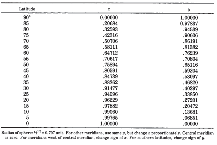
TABLE 42.— Mollweide projection: Rectangular coordinates for the 90th meridian — **TABLE 42**.— Mollweide projection: Rectangular coordinates for the 90th meridian