32. ECKERT IV AND VI PROJECTIONS #

SUMMARY #

Pseudocylindrical.
Equal-area.
Central meridian is a straight line; 180th meridians of Eckert IV are semicircles; all other meridians are equally spaced elliptical arcs on Eckert IV and sinusoidal curves on Eckert VI.
Parallels are unequally spaced straight lines, parallel to each other. Poles are straight lines half as long as the Equator.
Scale is true along latitudes 40°30’ N. and S. on Eckert IV and 49°16’ on Eckert VI.
Used for world maps.
Presented by Eckert in 1906.

HISTORY AND USAGE #

In 1906 Max Eckert (1868- 1938) of Kiel, Germany, presented a set of six new projections in which all the poles are lines half as long as the Equator, and in which all parallels of latitude are straight lines parallel to each other. The central meridian on each is also half the length of the Equator (Eckert, 1906). Numbers 4 and 6 are of most significance and are discussed here in detail.

Of the six projections, nos. 2, 4, and 6 are equal-area, and nos. 1, 3, and 5 are not equal-area but have equally spaced parallels. For nos. 1 and 2, the meridians are straight lines broken at the Equator, and those projections are therefore little more than novelties with graticules composed entirely of straight lines, but with unnecessary distortion especially at the Equator. The meridians on nos. 3 and 4 are elliptical arcs, while on 5 and 6 they are sinusoidal curves, with the exception of the straight central meridians, and (on 3 and 4) semicircular outer meridians.

No. 3, with equidistant parallels and elliptical arcs has occasionally been identified as the same as the Ortelius projection, named for the famous cartographer Abraham Ortelius who used a somewhat similar projection in 1570 for his world map. The border, the central meridian, and the parallels of the two projections are shown almost identically, and the meridians on each are equally spaced along the Equator. The shapes of most meridians, however, are different. On the Ortelius, they are circular arcs, semicircles for meridians at or more than 90° from the central meridian, and circular arcs intersecting the central meridian at the poles within 90° of the central meridian.

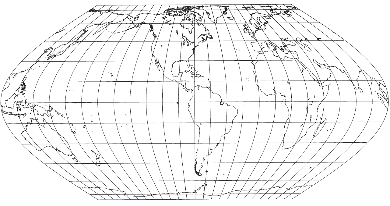
**FIGURE 56**.—Eckert IV projection. An equal-area pseudocylindrical with poles half the length of Equator. Outer meridians are semicircles; others are elliptical arcs.

The most commonly used of Eckert’s six projections have been his nos. 4 and 6, which are more often designated with Roman numerals IV and VI, respectively. In the United States, Eckert IV (fig. 56) has been used in several atlases to show climate and other themes. It has also been used as an inset on other maps, such as wall maps of the world by the National Geographic Society. It ranked third as an equal-area world map projection used in U.S. textbooks between 1940 and 1960, after the Goode Homolosine and Sinusoidal (Wong, 1965, p. 101). The Eckert VI (fig. 57) is much less used in the United States, although it has occasionally appeared in textbooks and atlases. It has been more popular in the Soviet Union, having been used for several world distribution maps in the 1937 Atlas Mira (World Atlas). An almost identical equal-area projection was presented by Karlheinz Wagner in 1932 and independently by V. V. Kavrayskiy in 1936; theirs does not require the iteration in computations which is required by Eckert VI (Maling, 1960, p.297; Snyder, 1977, p. 62).

**FIGURE 57**.— Eckert VI projection. Like figure 56, this is an equal-area pseudocylindrical projection with poles half the length of Equator. The meridians, however, are sinusoidal curves.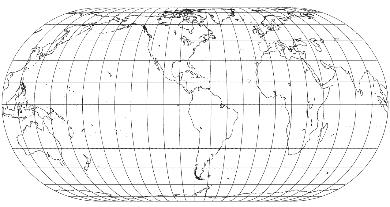

There have been numerous other pseudocylindrical projections with lines for poles, and Eckert’s were not the first, but they are the most popular. Some have been obtained by averaging a cylindrical projection with the Sinusoidal or Mollweide projection, and others are derived by stipulating that the poles be lines of some other length in proportion to the length of the Equator. Instead of the full sinusoid or full semiellipse, a portion of these curves or of some other mathematical curve has been used for the meridians (Snyder, 1977).

FEATURES #

The Eckert IV projection is bounded by two semicircles representing the 180th meridians and two straight lines connecting the ends of the semicircles. These straight lines represent the two poles, which are half the length of the Equator. Meridians are equally spaced semiellipses ranging in eccentricity from zero for the outer circular meridians to 1 for the straight central meridians. The parallels are straight lines parallel to the Equator and spaced to provide correct area within the border. They are therefore unequally spaced and closer together near the poles. There is a north-south stretching of shape at the Equator amounting to 40 percent relative to east-west dimensions. This stretching decreases along the central meridian to zero at latitudes 40°30’ N. and S. and becomes flattening beyond these parallels. The scale is correct only along these two parallels, and the only points free of distortion are at the intersection of these two points with the central meridian. Nearer the poles, the geographical features of the map are flattened in a north-south direction.

The Eckert VI projection of the world is bounded by two sinusoidal curves which have the same shape as the 90th meridians of the Sinusoidal projection. Like the border of the Eckert IV, these curved meridians are connected with two straight lines connecting the ends of the curves. These straight lines, half the length of the Equator, are the poles. The other meridians are equally spaced sinusoids, except for the straight central meridian, and the other parallels are straight and parallel to each other. To preserve area, the parallels must be unequally spaced, farther apart at the Equator than at the poles. As a result, there is a 29 percent north-south stretch at the Equator, relative to east-west dimensions. Other general comments concerning distortion of the Eckert IV apply to Eckert VI, but the latitudes of true scale are 49°16’ N. and S.

These projections are for world maps, not regional maps, and there is no need for the ellipsoidal forms.

FORMULAS FOR THE SPHERE #

The forward formulas for both Eckert IV and Eckert VI require iteration. Given $R, \lambda_0, \phi,$ and $\lambda$, to find $x$ and $y$ (see Eckert IV numerical examples and Eckert VI numerical examples):

Eckert IV:

$$ \begin{align} x &= \{2/[\pi(4+\pi)]^{1/2}\}R(\lambda-\lambda_0)(1+\cos\theta) \tag{32-1} \cr &= 0.4222382\,R(\lambda-\lambda_0)(1+\cos\theta) \tag{32-1a} \end{align} $$

$$ \begin{align} y &=2[\pi/(4+\pi)]^{1/2}R\sin\theta \tag{32-2} \cr &=1.3265004\,R\sin\theta \tag{32-2a} \end{align} $$

where

$$ \theta+\sin\theta+2\sin\theta = (2+\pi/2)\sin\phi \tag{ 32-3 } $$

The X axis coincides with the Equator, x increasing easterly, and the Y axis coincides with the central meridian, y increasing northerly. Angle $\theta$ is a parametric angle, not a polar coordinate. Equation (32-3) may be solved with rapid convergence (but slow at the poles) using a Newton-Raphson iteration consisting of the following instead of (32-3):

$$ \begin{align} \Delta\theta = &-[\theta+\sin\theta\cos\theta+2\sin\theta-(2+\pi/2)\sin\phi]/ \cr &[2\cos\theta(1+\cos\theta)] \end{align} \tag{ 32-4 } $$

With $(\phi/2)$ as the first trial $\theta$, $\Delta\theta$ is calculated from (32-4), this value is added to the preceding $\theta$ to obtain the next trial $\theta$, and the calculation is repeated with (32-4) until $\Delta\theta$ is less than a predetermined convergence value. Note that all these formulas are in terms of radians.

Eckert VI:

$$ x = R(\lambda-\lambda_0)(1+\cos\theta)/(2+\pi)^{1/2} \tag{ 32-5 } $$

$$ y = 2R\theta/(2+\pi)^{1/2} \tag{ 32-6 } $$

where

$$ \theta+\sin\theta = (1+\pi/2)\sin\phi \tag{ 32-7 } $$

Axes are as described above for Eckert IV; $\theta$ is parametric, but not the same as $\theta$ for Eckert IV. Equation (32-7) may be replaced with the following Newton-Raphson iteration, treated in the same manner as equation (32-4) for Eckert IV, but with $\phi$ as the first trial $\theta$:

$$ \Delta\theta=-[\theta+\sin\theta-(1+\pi/2)\sin\phi]/(1+\cos\theta) \tag{ 32-8 } $$

For the inverse formulas, given $R, \lambda_0, x,$ and $y$, to find $\phi$ and $\lambda$, no iteration is required:

Eckert IV:

$$ \begin{align} \theta &= \arcsin[y(4+\pi)^{1/2}/(2\pi^{1/2}R)] \tag{32-9} \cr &= \arcsin[y/(1.3265004R)] \tag{32-9a} \end{align} $$

$$ \phi = \arcsin[(\theta+\sin\theta\cos\theta+2\sin\theta)/(2+\pi/2)] \tag{ 32-10 } $$

$$ \begin{align} \lambda &= \lambda_0 + [\pi(4+\pi)]^{1/2}x/[2R(1+\cos\theta)] \tag{32-11} \cr &= \lambda_0 + x/[0.4222382R(1+\cos\theta)] \tag{32-11a} \end{align} $$

Eckert VI:

$$ \theta = (2+\pi)^{1/2}y/(2R) \tag{ 32-12 } $$

$$ \phi = \arcsin[(\theta+\sin\theta)/(1+\pi/2)] \tag{ 32-13 } $$

$$ \lambda = \lambda_0 + (2+\pi)^{1/2}x/[R(1+\cos\theta)] \tag{ 32-14 } $$

Table 43 lists the rectangular coordinates of the 90th meridian for a sphere of radius $[(4+\pi)^{1/2}/(2\pi^{1/2})]$ for Eckert IV and radius $[(2+\pi)^{1/2}/\pi^{1/2}]$ for Eckert VI, to make maximum values equal to 1.0. The x coordinates for other meridians are proportional, and y coordinates are constant for a given latitude.

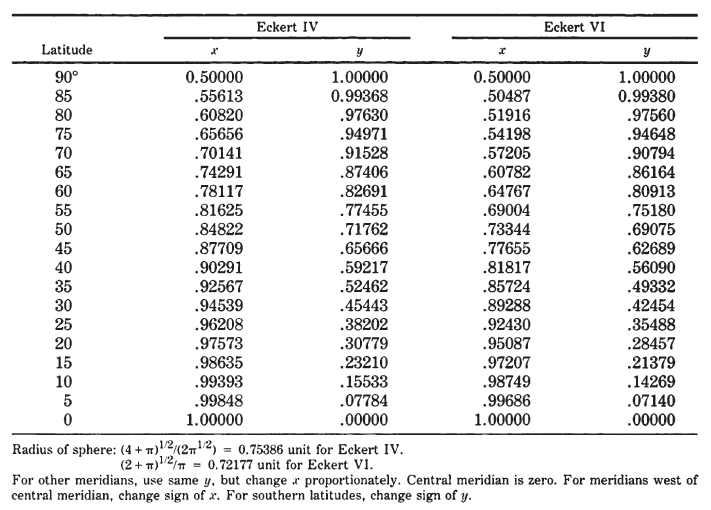
**TABLE 43**.—Eckert IV and VI projections: Rectangular coordinates for 90th meridian