PSEUDOCYLINDRICAL AND MISCELLANEOUS MAP PROJECTIONS #

29. VAN DER GRINTEN PROJECTION #

SUMMARY #

Neither equal-area nor conformal. Not pseudocylindrical.
Shows entire globe enclosed in a circle.
Central meridian and Equator are straight lines.
All other meridians and parallels are arcs of circles.
A curved modification of the Mercator projection, with great distortion in the polar areas.
Equator is true to scale.
Used for world maps.
Used only in the spherical form.
Presented by van der Grinten in 1904.

HISTORY, FEATURES, AND USAGE #

In a 1904 issue of a German geographical journal, Alphons J. van der Grinten (1852-?) of Chicago presented four projections showing the entire Earth. Aside from having a straight Equator and central meridian, three of the projections consist of arcs of circles for meridians and parallels; the other projection has straight-line parallels. The projections are neither conformal nor equal-area (van der Grinten, 1904; 1905). They were patented in the United States by van der Grinten in 1904.

The best-known Van der Grinten projection, his first (fig. 52), shows the world in a circle and was invented in 1898. It is designed for use in the spherical form only. There are no special features to preserve in an ellipsoidal form. It has been used by the National Geographic Society for their standard world map since 1943, printed at various scales and with the central meridian either through America or along the Greenwich meridian; this use has prompted others to employ the projection. The U.S. Department of Agriculture adopted the projection as the base map for economic data in the 1940’s, and this led to frequent use in geography textbooks (Wong, 1965, p. 117). The USGS has used one of the National Geographic maps as a base for a four-sheet set of maps of World Subsea Mineral Resources, 1970, one at a scale of 1:60,000,000 and three at 1:39,283,200 (a scale used by the National Geographic), and for three smaller maps in the National Atlas (USGS, 1970, p. 150-151, 332-335). All the USGS maps have a central meridian of long. 85° W., passing through the United States.

FIGURE 52.— Van der Grinten projection. A projection resembling Mercator, but not conformal. Used by USGS for special world maps, modifying a base map prepared by the national Geographic Society. This illustration is prepared by computer.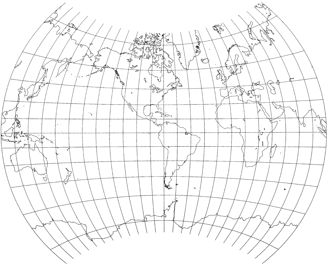 — **FIGURE 52**.— Van der Grinten projection. A projection resembling Mercator, but not conformal. Used by USGS for special world maps, modifying a base map prepared by the national Geographic Society. This illustration is prepared by computer.

Van der Grinten emphasized that this projection blends the Mercator appearance with the curves of the Mollweide, an equal-area projection described later. He included a simple graphical construction and limited formulas showing the mathematical coordinates along the central meridian, the Equator, and the outer (180th) meridian. The meridians are equally spaced along the Equator, but the spacing between the parallels increases with latitude, so that the 75th parallels are shown about halfway between the Equator and the respective poles. Because of the polar exaggerations, most published maps using the Van der Grinten projection do not extend farther into the polar regions than the northern shores of Greenland and the outer rim of Antarctica.

The National Geographic Society prepared the base map graphically. General mathematical formulas have been published in recent years and are only useful with computers, since they are fairly complex for such a simply drawn projection (O’Keefe and Greenberg, 1977; Snyder, 1979b).

GEOMETRIC CONSTRUCTION #

The meridians are circular arcs equally spaced on the Equator and joined at the poles. For parallels, referring to figure 53, semicircle CDB is drawn centered at A. Diagonal CD is drawn. Point E is marked so that the ratio of EA to AD is the same as the ratio of the latitude to 90°. Line FE is drawn parallel to CB, and FB and GB are connected. At H, the intersection of GB and AD, JHL is drawn parallel to CB. A circular arc, representing the parallel of latitude, is then drawn through JKL.

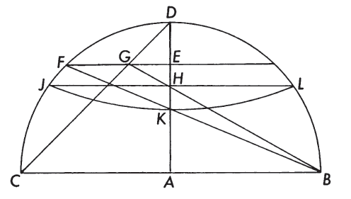
FORMULAS FOR THE SPHERE #

The general formulas published are in two forms. Both sets give identical results, but the 1979 formulas are somewhat shorter and are given here with some rearrangement and addition of new inverse equations. For the forward calculations, given $R, \lambda_0, \phi,$ and $\lambda$ (giving true scale along the Equator), to find $x$ and $y$ (see numerical examples):

$$ x = \pm\pi R\{A(G-P^2)+[A^2(G-P^2)^2-(P^2+A^2)(G^2-P^2)]^{1/2}\}/(P^2+A^2) \tag{ 29-1 } $$

taking the sign of $(\lambda-\lambda_0)$. Note that $(\lambda-\lambda_0)$ must fall between +180° and -180°; if necessary, 360° must be added or subtracted. The X axis lies along the Equator, x increasing easterly, while the Y axis coincides with the central meridian $\lambda_0$.

$$ y=\pm\pi R\{P Q - A[(A^2+1)(P^2+A^2)-Q^2]^{1/2}\}/(P^2+A^2) \tag{ 29-2 } $$

taking the sign of $\phi$,

where

$$ A = ½|\pi/(\lambda-\lambda_0)-(\lambda-\lambda_0)/\pi | \tag{ 29-3 } $$

$$ G = \cos\theta/(\sin\theta+\cos\theta-1) \tag{ 29-4 } $$

$$ P = G(2/\sin\theta-1) \tag{ 29-5 } $$

$$ \theta = \arcsin|2\phi/\pi| \tag{ 29-6 } $$

$$ Q = A^2+G \tag{ 29-6a } $$

But if $\phi = 0$ or $\pm90°$, or $\lambda = \lambda_0$, these equations are indeterminate. In that case, if $\phi=0$,

$$ x = R(\lambda-\lambda_0) \tag{ 29-7 } $$

and

$$ y = 0 $$

or if $\lambda=\lambda_0$ or $\phi = \pm90^\circ$

$$ x = 0 $$

and

$$ y=\pm\pi R\tan(\theta/2) \tag{ 29-8 } $$

taking the sign of $\phi$. It may be noted that absolute values (symbol $|\thinspace|$ ) are used in several cases. The origin is at the center $(\phi = 0, \lambda = \lambda_0)$.

For the inverse equations, given $R, \lambda_0, x,$ and $y,$ to find $\phi$ and $\lambda$: Because of the complications involved, the equations are given in the order of use. This is closely based upon a recent, noniterative algorithm by Rubincam (1981):

$$ X = x/(\pi R) \tag{ 29-9 } $$

$$ Y = y/(\pi R) \tag{ 29-10 } $$

$$ c_1 = -|Y|(1+X^2+Y^2) \tag{ 29-11 } $$

$$ c_2 = c_1 - 2Y^2+X^2 \tag{ 29-12 } $$

$$ c_3 = -2c_1+ 1 + 2Y^2+(X^2+Y^2)^2 \tag{ 29-13 } $$

$$ d = Y^2/c_3 + (2c_2^3/c_3^3-9c_1c_2/c_3^2)/27 \tag{ 29-14 } $$

$$ a_1 = (c_1-c_2^2/3c_3)/c_3 \tag{ 29-15 } $$

$$ m_1 = 2(-a_1/3)^{1/2} \tag{ 29-16 } $$

$$ \theta_1 = (1/3)\arccos(3d/a_1m_1) \tag{ 29-17 } $$

$$ \phi = \pm\pi[-m_1\cos(\theta_1+\pi/3)-c_2/3c_3] \tag{ 29-18 } $$

taking the sign of $y$.

$$ \lambda = \pi\{X^2+Y^2-1+[1+2(X^2-Y^2)+(X^2+Y^2)^2]^{1/2}\}/2X+\lambda_0 \tag{ 29-19 } $$

but if $X = 0$, equation (29- 19) is indeterminate. Then

$$ \lambda=\lambda_0 \tag{ 29-20 } $$

The formulas for scale factors are quite lengthy and are not included here. Rectangular coordinates are given in table 41 for a map of the world with unit radius of the outer circle. or $R = 1/\pi$. The longitude is measured from the central meridian. Only one quadrant of the map is given, but the map is symmetrical about both X and Y axes.

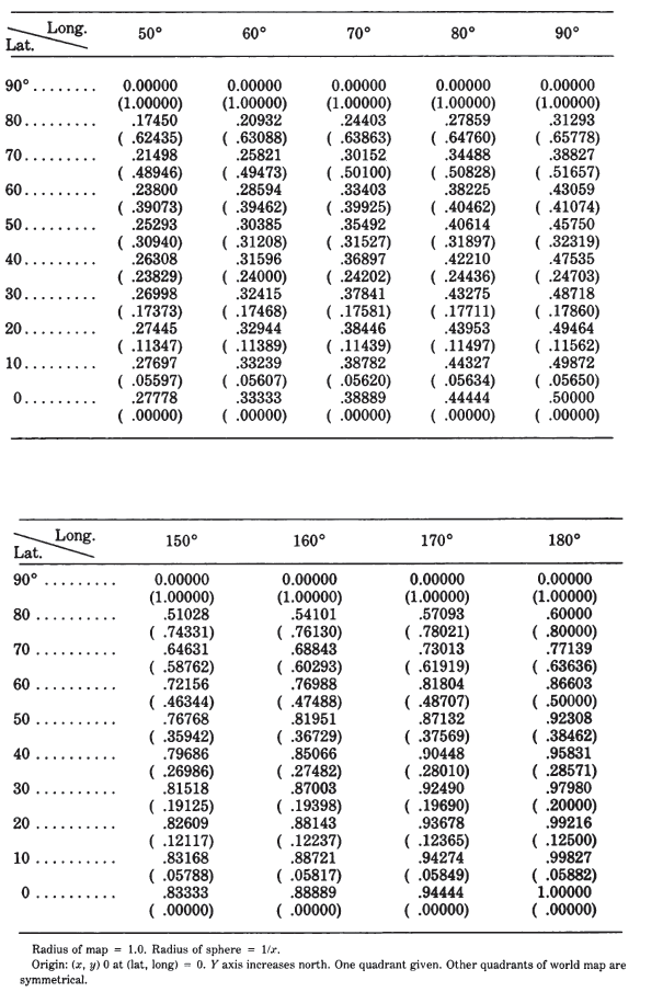
TABLE 41.— Van der Grinten projection: Rectangular coordinates — **TABLE 41**.— Van der Grinten projection: Rectangular coordinates

30. SINUSOIDAL PROJECTION #

SUMMARY #

Pseudocylindrical projection.
Equal-area.
Central meridian is a straight line; all other meridians are shown as equally spaced sinusoidal curves.
Parallels are equally spaced straight lines, parallel to each other. Poles are points.
Scale is true along central meridian and all parallels.
Used for world maps with single central meridian or in interrupted form with
several central meridians.
Used for maps of South America and Africa.
Used since the mid-16th century.

HISTORY #

There is an almost endless number of possible projections with horizontal straight lines for parallels of latitude and curved lines for meridians. They are sometimes called pseudocylindrical because of their partial similarity to cylindrical projections. Scores of such projections have been presented, purporting various special advantages, although several are strikingly similar to other members of the group (Snyder, 1977). While there were rudimentary projections with straight parallels used as early as the 2nd century B.C. by Hipparchus, the first such projection still used for scientific mapping of the sphere is the Sinusoidal.

This projection (fig. 54) used for world maps as well as maps of continents and other regions, especially those bordering the Equator, has been given many names after various presumed originators, but it is most frequently called by the name used here. Among the first to show the Sinusoidal projection was Jean Cossin of Dieppe, who used it for a world map of 1570. In addition, it was used by Jodocus Hondius for maps of South America and Africa in some of his editions of Mercator’s atlases of 1606-1609. This is probably the basis for one of the names of the projection: The Mercator Equal-Area. Nicolas Sanson (1600-67) of France used it in about 1650 for maps of continents, while John Flamsteed (1646-1719) of England later used it for star maps. Thus, the name “Sanson-Flamsteed” has often been applied to the Sinusoidal projection, even though they were not the originators (Keuning, 1955, p. 24; Deetz and Adams, 1934, p. 161).

**FIGURE 54**.— Interrupted Sinusoidal projection as used by USGS. The oldest pseudocylindrical projection, it shows areas correctly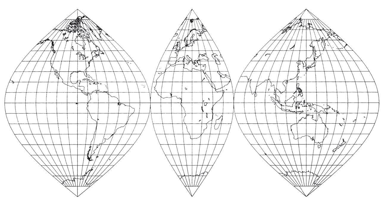

While maps of North America are no longer drawn to the Sinusoidal, South America and Africa are still shown on this projection in recent Rand McNally atlases.

FEATURES AND USAGE #

The simplicity of construction, either graphically or mathematically, combined with the useful features obtained, make the Sinusoidal projection not only popular to use, but a popular object of study for interruptions, transformations, and combination with other projections.

On the normal Sinusoidal projection, the parallels of latitude are equally spaced straight parallel lines, and the central meridian is a straight line crossing the parallels perpendicularly. The Equator is marked off from the central meridian equidistantly for meridians at the same scale as the latitude markings on the central meridian, so the Equator for a complete world map is twice as long as the central meridian. The other parallels of latitude are also marked off for meridians in proportion to the true distances from the central meridian. The meridians connect these markings from pole to pole. Since the spacings on the parallels are proportional to the cosine of the latitude, and since parallels are equally spaced, the meridians form curves which may be called cosine, sine,or sinusoidal curves; hence, the name.

Areas are shown correctly. There is no distortion along the Equator and central meridian, but distortion becomes pronounced near the outer meridians, especially in the polar regions.

Because of this distortion, J. Paul Goode (1862-1932) of the University of Chicago developed an interrupted form of the Sinusoidal in 1916 with several meridians chosen as central meridians without distortion and a limited expanse east and west for each section. The central meridians may be different for Northern and Southern Hemispheres and may be selected to minimize distortion of continents or of oceans instead. Ultimately, Goode combined the portion of the interrupted Sinusoidal projection between about lats. 40° N. and S. with the portions of the Mollweide or Homolographic projection (described later) not in this zone, to produce the Homolosine projection used in Rand McNally’s Goode’s Atlas (Goode, 1925).

In 1927, the Sinusoidal was shown interrupted in three symmetrical segments in the Nordisk Världs Atlas, Stockholm, serving as the base for the Sinusoidal as shown in Deetz and Adams (1934, p. 161). It is this interrupted form which served in turn as the base for a three-sheet set by the USGS in 1978 at a scale of 1:20,000,000, entitled Map of Prospective Hydrocarbon Provinces of the World. With interruptions occurring at longs. 160° W., 20° W., and 60° E., and the three central meridians equidistant from these limits, the sheets show (1) North and South America; (2) Europe, West Asia, and Africa; and (3) East Asia, Australia, and the Pacific; respectively. The maps extend pole to pole, but no data are shown for Antarctica. An inset of the Arctic region at the same scale is drawn to the polar Lambert Azimuthal Equal-Area projection. A similar map is being prepared by the USGS showing sedimentary basins of the world.

The Sinusoidal projection is normally used in the spherical form, adequate for the usual small-scale usage, but the ellipsoidal form has been used for topographic mapping in Ecuador (C. J. Mugnier, pers. comm., 1985).

FORMULAS FOR THE SPHERE #

The formulas for the Sinusoidal projection are perhaps the simplest of those for any projection described in this bulletin, except for the Equidistant Cylindrical. For the forward case, given $R, \lambda_0, \phi,$ and $\lambda$ to find $x$ and $y$ (see numerical examples):

$$ x = R(\lambda-\lambda_0)\cos\phi \tag{ 30-1 } $$

$$ y = R\phi \tag{ 30-2 } $$

$$ h = [1+(\lambda-\lambda_0)^2\sin^2\phi]^{1/2} \tag{ 30-3 } $$

$$ k = 1.0 $$

$$ \theta' = \arcsin(1/h) \tag{ 30-4 } $$

$$ \omega = 2\arctan|½(\lambda-\lambda_0)\sin\phi| \tag{ 30-5 } $$

where $\theta’$ is the angle of intersection of a given meridian and parallel (see equation (4-14)), and $h, k,$ and $\omega$ are other distortion factors as previously used. The X axis coincides with the Equator, with x increasing easterly, while the Y axis follows the central meridian $\lambda_0$, y increasing northerly. It is necessary to adjust $(\lambda-\lambda_0)$, if it falls outside the range ±180°, by adding or subtracting 360°. For the interrupted form, values of x are calculated for each section with respect to its own central meridian $\lambda_0$.

In equations (30-1) through (30-5), radians must be used, or $\phi$ and $\lambda$ in degrees must be multiplied by $\pi/180^\circ$.

For the inverse formulas, given $R, \lambda_0, x,$ and $y$, to find $\phi$ and $\lambda$:

$$ \phi = y/R \tag{ 30-6 } $$

$$ \lambda = \lambda_0+x/(R\cos\phi) \tag{ 30-7 } $$

but if $\phi = \pm\pi/2$, equation (30-7) is indeterminate, and $\lambda$ may be given an arbitrary value such as $\lambda_0$.

FORMULAS FOR THE ELLIPSOID #

The ellipsoidal form may be made by spacing parallels along the central meridian(s) true to scale for the ellipsoid and meridians along each parallel also true to scale. The projection remains equal-area, while the parallels are not quite equally spaced, and the meridians are no longer perfect sinusoids. Specifically, given $a, e, \lambda_0, \phi,$ and $\lambda$, to find $x$ and $y$ (see numerical examples):

$$ x = a(\lambda-\lambda_0)\cos\phi/(1-e^2\sin^2\phi)^{1/2} \tag{ 30-8 } $$

$$ y = M \tag{ 30-9 } $$

where

$$ \begin{align} M = a[&(1-e^2/4-3e^4/64-5e^6/256-\dots)\phi \\ -&(3e^2/8+3e^4/32+45e^6/1024+\dots)\sin{2\phi} \\ +&(15e^4/256+45e^6/1024+\dots)\sin{4\phi} - (35e^6/3072+\dots)\sin{6\phi}+\dots] \end{align} \tag{ 3-21 } $$

Axes are the same as those for the spherical form above.

For the inverse formulas, given $a, e, \lambda_0, x,$ and $y$, to find $\phi$ and $\lambda$:

$$ \begin{align} \phi = \mu &+ (3e_1/2-27e_1^3/32+\dots)\sin{2\mu}+(21e_1^2/16-55e_1^4/32+\dots)\sin{4\mu} \\ &+ (151e_1^3/96-\dots)\sin{6\mu}+(1097e_1^4/512-\dots)\sin{8\mu}+\dots \end{align} \tag{ 3-26 } $$

where

$$ e_1 = [1-(1-e^2)^{1/2}]/[1+(1-e^2)^{1/2}] \tag{ 3-24 } $$

$$ \mu=M/[a(1-e^2/4-3e^4/64-5e^6/256-\dots)] \tag{ 7-19 } $$

and

$$ M = y \tag{ 30-10 } $$

Then

$$ \lambda=\lambda_0+x(1-e^2\sin^2\phi)^{1/2}/(a\cos\phi) \tag{ 30-11 } $$

but if $\phi = \pm\pi/2$, equation (30-11) is indeterminate, and $\lambda$ may be given an arbitrary value such as $\lambda_0$.

31. MOLLWEIDE PROJECTION #

SUMMARY #

Pseudocylindrical.
Equal-area.
Central meridian is a straight line; 90th meridians are circular arcs; all other meridians are equally spaced elliptical arcs.
Parallels are unequally spaced straight lines, parallel to each other. Poles are points.
Scale is true along latitudes 40°44’ N. and S.
Used for world maps with single central meridian or in interrupted form with several central meridians.
Inspiration for several other projections.
Presented by Mollweide in 1805.

HISTORY AND USAGE #

The second oldest pseudocylindrical projection which is still in use (after the Sinusoidal) was presented by Carl B. Mollweide (1774-1825) of Halle, Germany, in 1805 (Mollweide, 1805). It is an equal-area projection of the Earth within an ellipse. It has had a profound effect on world map projections in the 20th century, especially as an inspiration for other important projections. It lay dormant until J. Babinet reintroduced it in 1857 under the name “homalographic.” It has been called Babinet’s Equal-Surface or the Elliptical projection, but it is most often called the Mollweide, Homalographic, or Homolographic.

J. Paul Goode, after interrupting the Sinusoidal projection, made similar interruptions of the Mollweide in 1916 to minimize distortion of continents or oceans. Ultimately he combined them to produce the Homolosine projection.

Other projections directly inspired by the Mollweide have been the Van der Grinten, described earlier, and the Boggs Eumorphic, in which the y coordinates of the Sinusoidal and Mollweide are arithmetically averaged, and the x coordinates are derived to maintain equality of area (Boggs, 1929). J. Fairgrieve in 1928 (Steers, 1970, p. 172) was the first of several to use the oblique aspect, and John Bartholomew applied the name “Atlantis” to a transverse Mollweide centered on the Atlantic Ocean and used as the frontispiece in The Times Atlas of 1958. Allen K. Philbrick (1953) combined the Sinusoidal and Mollweide in a manner different from the Goode Homolosine, using both normal and oblique aspects. Less direct inspiration by the Mollweide has led to several other projections, especially pseudocylindrical, some of which have lines for poles.

Some other projections showing the world in an ellipse, especially the Hammer and the Briesemeister, originate from the Lambert Azimuthal Equal-Area projection, not the Mollweide. Another projection occasionally seen is identical with the Mollweide, except that the parallels are equally spaced, and therefore the projection is not equal-area. It was first used in a rudimentary form in the 16th century.

FEATURES #

Unlike the Sinusoidal projection, which has been satisfactorily used for continental maps, the Mollweide projection (fig. 55) is normally used as a world map, and occasionally for a very large region such as the Pacific Ocean. This is because only two points on the Mollweide are completely free of distortion unless the projection is interrupted. These are the points at latitudes 40°44'12" N. and S. on the central meridian(s).

FIGURE 55.— Mollweide projection. An equal-are projection of the world bounded by an ellipse and the basis for several other projections. — **FIGURE 55**.— Mollweide projection. An equal-are projection of the world bounded by an ellipse and the basis for several other projections.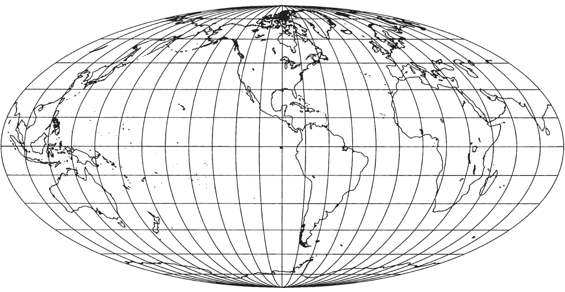

The world is shown in an ellipse with the Equator, its major axis, twice as long as the central meridian, its minor axis. The meridians 90° east and west of the central meridian form a complete circle. All other meridians are elliptical arcs which, with their opposite numbers on the other side of the central meridian, form complete ellipses which meet at the two poles. The central meridian is the major axis of meridian ellipses less than 90° from it, and a portion of the Equator is the minor axis. Meridians greater than 90° have the reverse arrangement for their axes. Meridians are equally spaced along the Equator and along all other parallels. The 90th meridians form a circle.

The parallels of latitude are straight parallel lines, but they are not equally spaced. Their spacing may be determined from the facts that the projection is equal-area and that the 90th meridians are circular. As a result, the regions along the Equator are stretched 23 percent in a north-south direction relative to east-west dimensions. This stretching decreases along the central meridian to zero at the 40°44’ latitudes, and becomes compression nearer the poles. The distortion near the outer meridians is considerable at high latitudes, but less than that on the Sinusoidal. The distortion along the Equator led Bromley (1965) to propose flattening the projection in a north-south direction and expanding east-west, to provide an Equator free of distortion, but the Equator thereby becomes 2.47 times as long as the central meridian.

Because the Mollweide projection is normally used at a small scale, there is little justification for an ellipsoidal form.

FORMULAS FOR THE SPHERE #

The forward formulas for the Mollweide require iteration, but they are otherwise relatively simple. Given $R, \lambda_0, \phi,$ and $\lambda$, to find $x$ and $y$ (see numerical examples):

$$ x = (8^{1/2}/\pi)R(\lambda-\lambda_0)\cos\theta \tag{ 31-1 } $$

$$ y = 2^{1/2}R\sin\theta \tag{ 31-2 } $$

where

$$ 2\theta+\sin2\theta = \pi\sin\phi \tag{ 31-3 } $$

The X axis coincides with the Equator, x increasing easterly, and the Y axis coincides with the central meridian, y increasing northerly. Angle $\theta$ is not a polar coordinate here; it is a parametric angle, geometrically the angle as seen from the center of the map between the Equator and the position of latitude $\phi$ on the 90th meridian circle.

Equation (31-3) may be solved with rapid convergence (but slow at the poles) using a Newton-Raphson iteration consisting of the following instead of (31-3):

$$ \Delta\theta' = -(\theta'+\sin\theta'-\pi\sin\phi)/(1+\cos\theta') \tag{ 31-4 } $$

With $\phi$ as the first trial $\theta’$, $\Delta\theta’$ is calculated from (31-4), this value is added to the preceding trial $\theta’$ to obtain the next trial $\theta’$, and the calculation is repeated with (31-4) until $\Delta\theta’$ is less than a predetermined convergence value. Then, using the final $\theta’$, $\theta$ is calculated as follows:

$$ \theta = \theta'/2 \tag{ 31-5 } $$

Note that all these formulas are in terms of radians. For the inverse formulas, given $R, \lambda_0, x,$ and $y$, to find $\phi$ and $\lambda$, no iteration is required:

$$ \theta = \arcsin[y/(2^{1/2}R)] \tag{ 31-6 } $$

$$ \phi = \arcsin[(2\theta+\sin{2\theta})/\pi] \tag{ 31-7 } $$

$$ \lambda = \lambda_0+\pi x/(8^{1/2}R\cos\theta) \tag{ 31-8 } $$

If $\phi$ is ±90°, equation (31-8) is indeterminate, but $\lambda$ may be made $\lambda_0$. Table 42 lists the rectangular coordinates of the 90th meridian for a sphere of radius $(1/2^{1/2})$, to make the maximum values equal to 1.0. The $x$ coordinates for other meridians are proportional, and $y$ coordinates are constant for a given latitude.

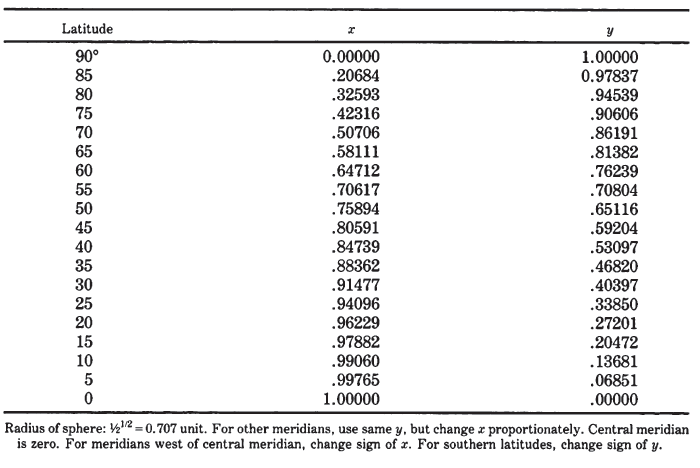
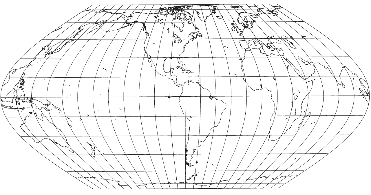
TABLE 42.— Mollweide projection: Rectangular coordinates for the 90th meridian — **TABLE 42**.— Mollweide projection: Rectangular coordinates for the 90th meridian

32. ECKERT IV AND VI PROJECTIONS #

SUMMARY #

Pseudocylindrical.
Equal-area.
Central meridian is a straight line; 180th meridians of Eckert IV are semicircles; all other meridians are equally spaced elliptical arcs on Eckert IV and sinusoidal curves on Eckert VI.
Parallels are unequally spaced straight lines, parallel to each other. Poles are straight lines half as long as the Equator.
Scale is true along latitudes 40°30’ N. and S. on Eckert IV and 49°16’ on Eckert VI.
Used for world maps.
Presented by Eckert in 1906.

HISTORY AND USAGE #

In 1906 Max Eckert (1868- 1938) of Kiel, Germany, presented a set of six new projections in which all the poles are lines half as long as the Equator, and in which all parallels of latitude are straight lines parallel to each other. The central meridian on each is also half the length of the Equator (Eckert, 1906). Numbers 4 and 6 are of most significance and are discussed here in detail.

Of the six projections, nos. 2, 4, and 6 are equal-area, and nos. 1, 3, and 5 are not equal-area but have equally spaced parallels. For nos. 1 and 2, the meridians are straight lines broken at the Equator, and those projections are therefore little more than novelties with graticules composed entirely of straight lines, but with unnecessary distortion especially at the Equator. The meridians on nos. 3 and 4 are elliptical arcs, while on 5 and 6 they are sinusoidal curves, with the exception of the straight central meridians, and (on 3 and 4) semicircular outer meridians.

No. 3, with equidistant parallels and elliptical arcs has occasionally been identified as the same as the Ortelius projection, named for the famous cartographer Abraham Ortelius who used a somewhat similar projection in 1570 for his world map. The border, the central meridian, and the parallels of the two projections are shown almost identically, and the meridians on each are equally spaced along the Equator. The shapes of most meridians, however, are different. On the Ortelius, they are circular arcs, semicircles for meridians at or more than 90° from the central meridian, and circular arcs intersecting the central meridian at the poles within 90° of the central meridian.

**FIGURE 56**.—Eckert IV projection. An equal-area pseudocylindrical with poles half the length of Equator. Outer meridians are semicircles; others are elliptical arcs.

The most commonly used of Eckert’s six projections have been his nos. 4 and 6, which are more often designated with Roman numerals IV and VI, respectively. In the United States, Eckert IV (fig. 56) has been used in several atlases to show climate and other themes. It has also been used as an inset on other maps, such as wall maps of the world by the National Geographic Society. It ranked third as an equal-area world map projection used in U.S. textbooks between 1940 and 1960, after the Goode Homolosine and Sinusoidal (Wong, 1965, p. 101). The Eckert VI (fig. 57) is much less used in the United States, although it has occasionally appeared in textbooks and atlases. It has been more popular in the Soviet Union, having been used for several world distribution maps in the 1937 Atlas Mira (World Atlas). An almost identical equal-area projection was presented by Karlheinz Wagner in 1932 and independently by V. V. Kavrayskiy in 1936; theirs does not require the iteration in computations which is required by Eckert VI (Maling, 1960, p.297; Snyder, 1977, p. 62).

**FIGURE 57**.— Eckert VI projection. Like figure 56, this is an equal-area pseudocylindrical projection with poles half the length of Equator. The meridians, however, are sinusoidal curves.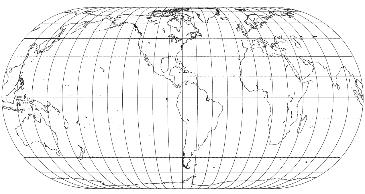

There have been numerous other pseudocylindrical projections with lines for poles, and Eckert’s were not the first, but they are the most popular. Some have been obtained by averaging a cylindrical projection with the Sinusoidal or Mollweide projection, and others are derived by stipulating that the poles be lines of some other length in proportion to the length of the Equator. Instead of the full sinusoid or full semiellipse, a portion of these curves or of some other mathematical curve has been used for the meridians (Snyder, 1977).

FEATURES #

The Eckert IV projection is bounded by two semicircles representing the 180th meridians and two straight lines connecting the ends of the semicircles. These straight lines represent the two poles, which are half the length of the Equator. Meridians are equally spaced semiellipses ranging in eccentricity from zero for the outer circular meridians to 1 for the straight central meridians. The parallels are straight lines parallel to the Equator and spaced to provide correct area within the border. They are therefore unequally spaced and closer together near the poles. There is a north-south stretching of shape at the Equator amounting to 40 percent relative to east-west dimensions. This stretching decreases along the central meridian to zero at latitudes 40°30’ N. and S. and becomes flattening beyond these parallels. The scale is correct only along these two parallels, and the only points free of distortion are at the intersection of these two points with the central meridian. Nearer the poles, the geographical features of the map are flattened in a north-south direction.

The Eckert VI projection of the world is bounded by two sinusoidal curves which have the same shape as the 90th meridians of the Sinusoidal projection. Like the border of the Eckert IV, these curved meridians are connected with two straight lines connecting the ends of the curves. These straight lines, half the length of the Equator, are the poles. The other meridians are equally spaced sinusoids, except for the straight central meridian, and the other parallels are straight and parallel to each other. To preserve area, the parallels must be unequally spaced, farther apart at the Equator than at the poles. As a result, there is a 29 percent north-south stretch at the Equator, relative to east-west dimensions. Other general comments concerning distortion of the Eckert IV apply to Eckert VI, but the latitudes of true scale are 49°16’ N. and S.

These projections are for world maps, not regional maps, and there is no need for the ellipsoidal forms.

FORMULAS FOR THE SPHERE #

The forward formulas for both Eckert IV and Eckert VI require iteration. Given $R, \lambda_0, \phi,$ and $\lambda$, to find $x$ and $y$ (see Eckert IV numerical examples and Eckert VI numerical examples):

Eckert IV:

$$ \begin{align} x &= \{2/[\pi(4+\pi)]^{1/2}\}R(\lambda-\lambda_0)(1+\cos\theta) \tag{32-1} \cr &= 0.4222382\,R(\lambda-\lambda_0)(1+\cos\theta) \tag{32-1a} \end{align} $$

$$ \begin{align} y &=2[\pi/(4+\pi)]^{1/2}R\sin\theta \tag{32-2} \cr &=1.3265004\,R\sin\theta \tag{32-2a} \end{align} $$

where

$$ \theta+\sin\theta+2\sin\theta = (2+\pi/2)\sin\phi \tag{ 32-3 } $$

The X axis coincides with the Equator, x increasing easterly, and the Y axis coincides with the central meridian, y increasing northerly. Angle $\theta$ is a parametric angle, not a polar coordinate. Equation (32-3) may be solved with rapid convergence (but slow at the poles) using a Newton-Raphson iteration consisting of the following instead of (32-3):

$$ \begin{align} \Delta\theta = &-[\theta+\sin\theta\cos\theta+2\sin\theta-(2+\pi/2)\sin\phi]/ \cr &[2\cos\theta(1+\cos\theta)] \end{align} \tag{ 32-4 } $$

With $(\phi/2)$ as the first trial $\theta$, $\Delta\theta$ is calculated from (32-4), this value is added to the preceding $\theta$ to obtain the next trial $\theta$, and the calculation is repeated with (32-4) until $\Delta\theta$ is less than a predetermined convergence value. Note that all these formulas are in terms of radians.

Eckert VI:

$$ x = R(\lambda-\lambda_0)(1+\cos\theta)/(2+\pi)^{1/2} \tag{ 32-5 } $$

$$ y = 2R\theta/(2+\pi)^{1/2} \tag{ 32-6 } $$

where

$$ \theta+\sin\theta = (1+\pi/2)\sin\phi \tag{ 32-7 } $$

Axes are as described above for Eckert IV; $\theta$ is parametric, but not the same as $\theta$ for Eckert IV. Equation (32-7) may be replaced with the following Newton-Raphson iteration, treated in the same manner as equation (32-4) for Eckert IV, but with $\phi$ as the first trial $\theta$:

$$ \Delta\theta=-[\theta+\sin\theta-(1+\pi/2)\sin\phi]/(1+\cos\theta) \tag{ 32-8 } $$

For the inverse formulas, given $R, \lambda_0, x,$ and $y$, to find $\phi$ and $\lambda$, no iteration is required:

Eckert IV:

$$ \begin{align} \theta &= \arcsin[y(4+\pi)^{1/2}/(2\pi^{1/2}R)] \tag{32-9} \cr &= \arcsin[y/(1.3265004R)] \tag{32-9a} \end{align} $$

$$ \phi = \arcsin[(\theta+\sin\theta\cos\theta+2\sin\theta)/(2+\pi/2)] \tag{ 32-10 } $$

$$ \begin{align} \lambda &= \lambda_0 + [\pi(4+\pi)]^{1/2}x/[2R(1+\cos\theta)] \tag{32-11} \cr &= \lambda_0 + x/[0.4222382R(1+\cos\theta)] \tag{32-11a} \end{align} $$

Eckert VI:

$$ \theta = (2+\pi)^{1/2}y/(2R) \tag{ 32-12 } $$

$$ \phi = \arcsin[(\theta+\sin\theta)/(1+\pi/2)] \tag{ 32-13 } $$

$$ \lambda = \lambda_0 + (2+\pi)^{1/2}x/[R(1+\cos\theta)] \tag{ 32-14 } $$

Table 43 lists the rectangular coordinates of the 90th meridian for a sphere of radius $[(4+\pi)^{1/2}/(2\pi^{1/2})]$ for Eckert IV and radius $[(2+\pi)^{1/2}/\pi^{1/2}]$ for Eckert VI, to make maximum values equal to 1.0. The x coordinates for other meridians are proportional, and y coordinates are constant for a given latitude.

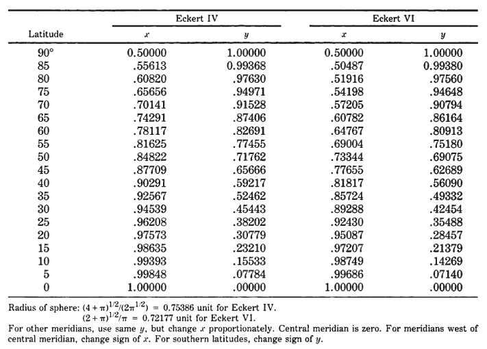
**TABLE 43**.—Eckert IV and VI projections: Rectangular coordinates for 90th meridian