2D Interpolation Functions #

Two-dimensional interpolation finds its way in many applications like image processing and digital terrain modeling. Here we will compare different interpolation strategies.

The purpose of the interpolation is to “densify” a sparse data set by creating intermediate points. For our examples we will take a 4 by 5 matrix and assign each value an arbitrary color. In the original matrix there are 3 by 4 intervals. We will divide each interval in N=100 points, creating a 300x400 pixel image.

Here is our initial matrix:

$$ V = \left[ \matrix {1 & 2 & 4 & 1 \cr 6 & 3 & 5 & 2 \cr 4 & 2 & 1 & 5 \cr 5 & 4 & 2 & 3 \cr 2 & 3 & 6 & 4 }\right] $$

For presenting the results we will use a color map: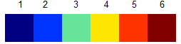
discrete color bar

or, as a continuous color bar: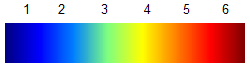

Method 1 - The Simple Way - Nearest Neighbor Interpolation #

The simplest interpolation strategy is just to take the value from the nearest data point. It could also be called “zero degree interpolation” and is described by the function:

$$ nni(x,y)=V_{round(x),round(y)} $$

The output matrix is simply generated by $M_{ij}=nni(i/N, j/N)$.

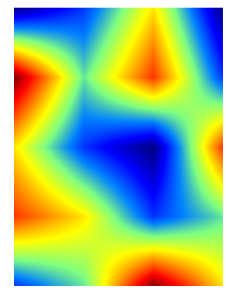
This is a color map of the resulting matrix: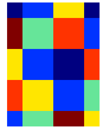

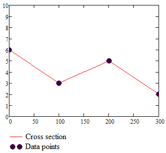
And below is a cross section going through second row of the original data set. It shows the initial data points and interpolated values: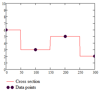

Looking at the cross section, notice the sudden jumps that translate into the sudden changes of color.

Although the method seems almost too simple, if the original data set is dense enough and the data points aren’t too noisy, this method can give acceptable results.

Method 2 - The Popular Way - Bilinear Interpolation #

This is one of the most popular methods. The interpolation function is linear in X and in Y (hence the name – bilinear). If we denote $\lfloor x \rfloor = floor(x)$ the largest integer not greater than $x$ and $ \lbrace x \rbrace = frac(x) = x-\lfloor x \rfloor$, the fractional part of $x$, then:

$$ \eqalign{ blin(x,y) =& (1-\{x\})(1-\{y\})V_{\lfloor x\rfloor,\lfloor y\rfloor} + \{x\}(1-\{y\})V_{\lfloor x\rfloor +1,\lfloor y\rfloor} \cr &+ (1-\{x\})\{y\}V_{\lfloor x\rfloor,\lfloor y\rfloor+1} + \{x\}\{y\}V_{\lfloor x\rfloor+1,\lfloor y\rfloor+1}\cr } $$

The resulting matrix is $ M_{ij}=blin(i/N,j/N) $. The color map representation is:

And the cross section:

Now, looking at the cross section, you can see that there are no sudden jumps (the interpolation function is continuous). There are however sudden changes in slope (in calculus parlance - the first derivative is not continuous) and those produce the diamond shaped artifacts in the color map.

Method 3 - The Wrong Way - Biquadratic Interpolation #

If a first degree (linear) function got us a continuous interpolation function but with a discontinuous derivative, maybe a second degree (called quadratic or parabolic) function will give us a better interpolation function.

I have encountered this method in the NGS GEOCON program and the oldest version I could find is in GEOID90 interpolation program.

Instead of using a linear function, this method uses a second degree function:

$$ qterp2(t,a) = a_0 + t(a_1-a_0)+ \frac 1 2t(t-1)(a_2-2a_1+a_0) $$

where t is in the range 0 to 2. It can be seen that $qterp2(0)=a_0$, $qterp2(1)=a_1$ and $qterp2(2)=a_2$.

These conditions uniquely define the coefficients of a second degree function so there is nothing we can do to force the first derivative to be continuous.

The one dimensional interpolation is expanded to two dimensions by making first 3 interpolations along the X axis with increasing Y values and then interpolating the resulting 3 values along the Y axis. The resulting color map is: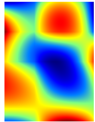

The cross section is: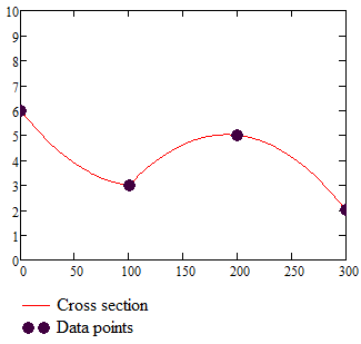

To better understand what’s going on let’s examine a one dimensional interpolation. We have 3 functions: $q_1$ going through the first 3 points, $q_2$ going through points 2, 3, 4 and $q_3$ going through points 3, 4, 5. Then we have the interpolation function that assembles pieces of each one:

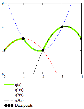
$$ q(x) = \cases {q_1(x) &if $x < 1$ \cr q_2(x) &if $1 \le x < 2$ \cr q_3(x) &if $x \ge 2$ } $$

The graph below shows how the interpolation function is assembled:

Discontinuities in the first derivative are even more pronounced than in the case of linear interpolation. The change from a linear function to a parabolic one doesn’t bring any obvious advantage. We still can have sharp transitions in the slope and the resulting surface looks even stranger than in the case of bilinear interpolation. The added complexity doesn’t bring any benefit.

For a more complete discussion of this algorithm see ¹

Method 4 - The Complicated Way - Bicubic Interpolation #

If we want slope continuity we have to go to one degree up to cubic functions. A bicubic function can be expressed as:

$$ bic(x, y, a) = \sum_{i=0}^3\sum_{j=0}^3 a_{ij}x^iy^j $$

or in matrix notation:

$$ bic(x, y, a) = [ \array{1 & x & x^2 & x^3} ]\left [ \matrix{a_{0\,0} & a_{0\,1} & a_{0\,2} & a_{0\,3} \cr a_{1\,0} & a_{1\,1} & a_{1\,2} & a_{1\,3} \cr a_{2\,0} & a_{2\,1} & a_{2\,2} & a_{2\,3} \cr a_{3\,0} & a_{3\,1} & a_{3\,2} & a_{3\,3} \cr } \right] \left [ \array {1 \cr y \cr y^2 \cr y^3} \right] $$

The challenge is to find the values of the 16 coefficients. They can be determined by solving a system of equations formed by:

4 equations for function values in each corner of the interpolation square
8 equations for partial derivatives in each corner of the interpolation square (4 in the x direction and 4 in the y direction)
4 equations for mixed derivatives in each corner of the interpolation square

The values for partial derivatives or mixed derivatives are estimated using differences between adjacent data points.

Now, solving a system of 16 equations for each interpolation square is not the best way to make a highly efficient algorithm. Fortunately it turns out that, if we write the 16 equations, the system can be written as

$$ W \left [ \array{a_{0\,0}\cr a_{1\,0}\cr a_{2\,0}\cr a_{3\,0}\cr a_{0\,1}\cr a_{1\,1}\cr a_{2\,1}\cr a_{3\,1}\cr a_{0\,2}\cr a_{1\,2}\cr a_{2\,2}\cr a_{3\,2}\cr a_{0\,3}\cr a_{1\,3}\cr a_{2\,3}\cr a_{3\,3}\cr} \right ] = \left [ \array {V_{0\,0}\cr V_{1\,0} \cr V_{0\,1} \cr V_{1\,1} \cr Vx_{0\,0}\cr Vx_{1\,0} \cr Vx_{0\,1} \cr Vx_{1\,1} \cr Vy_{0\,0}\cr Vy_{1\,0} \cr Vy_{0\,1} \cr Vy_{1\,1} \cr Vxy_{0\,0}\cr Vxy_{1\,0} \cr Vxy_{0\,1} \cr Vxy_{1\,1} \cr}\right] $$

where $V$ are the data points values, $Vx$ the partial derivative in the x direction, $Vy$ the partial derivative in the y direction and $Vxy$ the cross derivatives. The $W$ matrix is a fixed matrix that doesn’t depend on the data points. The values of the coefficients a can be found from:

$$ \left [ \array{a_{0\,0}\cr a_{1\,0}\cr a_{2\,0}\cr a_{3\,0}\cr a_{0\,1}\cr a_{1\,1}\cr a_{2\,1}\cr a_{3\,1}\cr a_{0\,2}\cr a_{1\,2}\cr a_{2\,2}\cr a_{3\,2}\cr a_{0\,3}\cr a_{1\,3}\cr a_{2\,3}\cr a_{3\,3}\cr} \right ] = W^{-1} \left [ \array {V_{0\,0}\cr V_{1\,0} \cr V_{0\,1} \cr V_{1\,1} \cr Vx_{0\,0}\cr Vx_{1\,0} \cr Vx_{0\,1} \cr Vx_{1\,1} \cr Vy_{0\,0}\cr Vy_{1\,0} \cr Vy_{0\,1} \cr Vy_{1\,1} \cr Vxy_{0\,0}\cr Vxy_{1\,0} \cr Vxy_{0\,1} \cr Vxy_{1\,1} \cr}\right] $$

The inverse of W can be pre-calculated and solving the system of equations reduces to “just” one matrix multiplication. For reference, here is the inverse of the W matrix:

$$ W^{-1} = \left [ \matrix { 1 & 0 & 0 & 0 & 0 & 0 & 0 & 0 & 0 & 0 & 0 & 0 & 0 & 0 & 0 & 0 \cr 0 & 0 & 0 & 0 & 1 & 0 & 0 & 0 & 0 & 0 & 0 & 0 & 0 & 0 & 0 & 0 \cr 0 & 0 & 0 & 0 & 0 & 0 & 0 & 0 & 0 & 0 & 0 & 0 & 1 & 0 & 0 & 0 \cr -3 & 3 & 0 & 0 & -2 & -1 & 0 & 0 & 0 & 0 & 0 & 0 & 0 & 0 & 0 & 0 \cr 2 & -2 & 0 & 0 & 1 & 1 & 0 & 0 & 0 & 0 & 0 & 0 & 0 & 0 & 0 & 0 \cr 0 & 0 & 0 & 0 & 0 & 0 & 0 & 0 & 1 & 0 & 0 & 0 & 0 & 0 & 0 & 0 \cr 0 & 0 & 0 & 0 & 0 & 0 & 0 & 0 & -3 & 3 & 0 & 0 & -2 & -1 & 0 & 0 \cr 0 & 0 & 0 & 0 & 0 & 0 & 0 & 0 & 2 & -2 & 0 & 0 & 1 & 1 & 0 & 0 \cr -3 & 0 & 3 & 0 & 0 & 0 & 0 & 0 & -2 & 0 & -1 & 0 & 0 & 0 & 0 & 0 \cr 0 & 0 & 0 & 0 & -3 & 0 & 3 & 0 & 0 & 0 & 0 & 0 & -2 & 0 & -1 & 0 \cr 9 & -9 & -9 & 9 & 6 & 3 & -6 & -3 & 6 & -6 & 3 & -3 & 4 & 2 & 2 & 1 \cr -6 & 6 & 6 & -6 & -3 & -3 & 3 & 3 & -4 & 4 & -2 & 2 & -2 & -2 & -1 & -1 \cr 2 & 0 & -2 & 0 & 0 & 0 & 0 & 0 & 1 & 0 & 1 & 0 & 0 & 0 & 0 & 0 \cr 0 & 0 & 0 & 0 & 2 & 0 & -2 & 0 & 0 & 0 & 0 & 0 & 1 & 0 & 1 & 0 \cr -6 & 6 & 6 & -6 & -4 & -2 & 4 & 2 & -3 & 3 & -3 & 3 & -2 & -1 & -2 & -1 \cr 4 & -4 & -4 & 4 & 2 & 2 & -2 & -2 & 2 & -2 & 2 & -2 & 1 & 1 & 1 & 1 \cr } \right] $$

You can find it also on the Wikipedia page for bicubic interpolation.

The resulting color map for our data set is: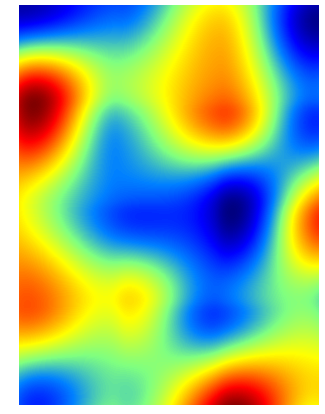

and the cross section: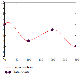

The interpolation function is indeed continuous and the slope is also continuous but it can have over and undershoots. They come from the rather arbitrary estimates we made for the partial derivatives - remember, they are assumed to be the difference between adjacent data points. Anyway, if you decide to use bicubic interpolation, these overshoots are a fact of life and you have to take it into account and rescale or truncate accordingly.

Method 5 - My Way - Constrained Bicubic Interpolation #

The bicubic algorithm can be modified by forcing the partial derivatives and cross derivatives to be 0 at each data point.

This simplifies the process of finding the bicubic coefficients and turns them simply into a weighting function:

$$ w(x,y) = x^2y^2(9-6x-6y+4x y) $$

The interpolation function becomes:

$$ \eqalign{ cbi(x,y) =& w(1-\{x\},1-\{y\})V_{\lfloor x\rfloor\,\lfloor y\rfloor} \cr &+w(\{x\}, 1-\{y\})V_{\lfloor x\rfloor+1\,\lfloor y\rfloor} \cr &+w(1-\{x\},\{y\})V_{\lfloor x\rfloor\,\lfloor y\rfloor+1} \cr &+w(\{x\}, \{y\})V_{\lfloor x\rfloor+1\,\lfloor y\rfloor+1} } $$

where $\lfloor x\rfloor$ and $\lbrace x \rbrace$ denote again the floor and fractional part functions, respectively.

The resulting matrix is $M_{i,j}=cbi(i/N,j/N)$. The color map representation is: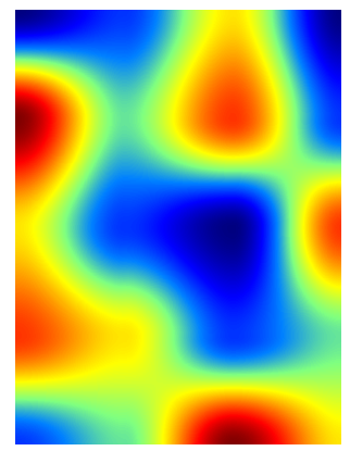

The cross section: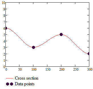

shows that the interpolation function is continuous with a continuous slope. Moreover, the slope is 0 in each data point and that prevents any over or undershoots.

If we look back at the bilinear interpolation method, the interpolation formula can be rewritten as:

but with a weighting function:

$$ w(x,y) = x \cdot y $$

That means we can switch between the constrained bicubic interpolation and bilinear interpolation by changing only the weighting function.

A historical note: I found this algorithm many years ago in a document suggesting how GPS receivers should interpolate the MSL height from a (very sparse) geoid model. Unfortunately I don’t remember the exact source and I couldn’t find any reference.

Show Me the Code #

The interp2.h file contains all the algorithms described above:

// Nearest neighbor interpolation
template<typename T>
void nni (const Matrix<T>& in, Matrix<T>& out)

// Bilinear interpolation
template<typename T>
void bilin (const Matrix<T>& in, Matrix<T>& out)

// Biquadratic interpolation
template<typename T>
void biquad (const Matrix<T>& in, Matrix<T>& out)

// Bicubic interpolation
template<typename T>
void bicube (const Matrix<T>& in, Matrix<T>& out)

// Constrained bicubic interpolation
template<typename T>
void cbi (const Matrix<T>& in, Matrix<T>& out)

They all need some matrix representation for the data. I very strongly recommend to use a professional matrix algebra package for any serious work. Do not roll out your own unless you are some kind of genius who likes reinventing the wheel. My personal preference is for Eigen but there are many to choose from.

That being said, the interp2.h file contains a very simple implementation of a Matrix class. It contains the absolute minimum of operations required by the interpolation algorithms. You can use it to get acquainted with the interpolation methods or if you cannot use a better matrix package.

There is also a sample project showing how to use these interpolation functions.

Conclusions #

I have presented the most common methods for two-dimensional interpolation. Choosing one over the other depends on the particular context but, needless to say, my favorite is method 5.

References #

NOAA Technical Memorandum NOS NGS 84 https://geodesy.noaa.gov/library/pdfs/NOAA_TM_NOS_NGS_0084.pdf ↩︎